Introduction to the Linear Model (MT8)
This week we will introduce the linear model as an overarching framework for understanding common statistical tools in the psychological sciences. You will learn about the most basic form of as statistical model, that is: DATA = MODEL + ERROR. The model part of this formula being our “best guess” given available information, and the error part being the imprecision or variance of that best guess from the observed data. The concepts introduced here are the fundamental building blocks for the more complex statistical models that we will construct in subsequent weeks, which allow us to add variables that might reduce (or explain) the variance around our “best guess”.
Learning outcomes
At the end of today’s workshop you should be able to do the following:
1.Build an empty model by calcuating the predicted values and the residuals
Calcuate error using sum of sqaures, variance, and standard deviation
Use lm() and anova() to test our calcaultions
Compare distributions of choice for Australia and Japan using Z-scores
Install required packages
install.packages("tidyverse")
install.packages("mosaic")
install.packages("ggplot2")
install.packages("sjlabelled")
Load required packages
The required packages are the same as the installed packages. Write the code needed to load the required packages in the below R chunk.
library("tidyverse")
library("mosaic")
library("ggplot2")
library("sjlabelled")
The WVS data
If you would like to have a quick recap on the data we will be working with, go to the World Value Survey site. Don’t download anything: http://www.worldvaluessurvey.org/WVSContents.jsp.
You can access the .rdata (R data file) file of the data here: https://github.com/thomcurran/PB130/raw/master/MT3/Workshop/WV6_Data_R_v20180912.rds. The file is called WV6_Data_R_v20180912.rds. The .rds extension is an R speicifc extension, most commonly we’ll work with .csv files.
Now we are going to open the file in R using RStudio or RStudio Server. Use the command below, but be sure to change the filepath to the one where you have put the WV6_Data_R_v20180912.rds file.
WVS <- readRDS("C:/Users/CURRANT/Dropbox/Work/LSE/PB130/MT8/Workshop/WV6_Data_R_v20180912.rds")

WVS$V2A <- as_character(WVS$V2A) # this saves the country varaible as a "character" variable (i.e., the names of th countries) rather than its default "numeric" value.
Case Study in Visulising Data: Perceptions of Choice in the Australia and Japan
Lets move on from the last workshop and look at one variable this week - perceptions of choice in life - and how we can use the mean and SD to make estimations about the likelihood of someone scoring above the middle value in each country. The perceptions of choice in life variable asks the question: “How much freedom of choice and control over own life” and is measured on a 1-10 scale:
- No choice at all
. . .
- A great deal of choice
I looked in the codebook and the perceptions of choice variable is listed as V55. So lets look for the variable and select it, then head the new dataframe entitled WVSchoice. Lets also select the country code variable, V2A, so we can use this to group the choice scores later. I have left some of the below code blank for you to fill the gap.
WVSchoice <-
  WVS %>%
  select(V55, V2A) # SELECT THE VARIABLES OF INTEREST HERE
head(WVSchoice)
## # A tibble: 6 x 2
## V55 V2A
## <labelled> <chr>
## 1 7 Algeria
## 2 6 Algeria
## 3 6 Algeria
## 4 6 Algeria
## 5 6 Algeria
## 6 4 AlgeriaLets now run the favstats() function to see what we are playing with for the choice variable (V55).
favstats()Just like other variables in this dataset, we need to edit the dataframe since the variable has values we can’t interpret like -5. While we are at it, lets also filter out Australia in the first instance as the country of interest. We can do that by using the filter() function.
WVSaus <-
WVSchoice %>%
filter(V55 >= "1" & V2A == c("Australia"))
WVSaus
## # A tibble: 1,459 x 2
## V55 V2A
## <labelled> <chr>
## 1 9 Australia
## 2 9 Australia
## 3 6 Australia
## 4 8 Australia
## 5 2 Australia
## 6 9 Australia
## 7 7 Australia
## 8 5 Australia
## 9 6 Australia
## 10 8 Australia
## # ... with 1,449 more rowsBox-plot, histogram, and descriptives.
The empty model
Lets begin to build an empty model for Australia. The first step in this process is to calcuate the mean and save it into the dataframe. Remeber, the mean is our “best guess” of what someone in Austrsalia would score on perceptions of choice given no other information. The mean is the empty model. It is the predicted score. We can calcualte and save the mean as an additional variable in our dataframe using the mutate() function.
WVSaus <-
  WVSaus %>%
  mutate(mean_choice = mean(V55))
WVSaus
## # A tibble: 1,459 x 3
## V55 V2A mean_choice
## <labelled> <chr> <dbl>
## 1 9 Australia 7.81
## 2 9 Australia 7.81
## 3 6 Australia 7.81
## 4 8 Australia 7.81
## 5 2 Australia 7.81
## 6 9 Australia 7.81
## 7 7 Australia 7.81
## 8 5 Australia 7.81
## 9 6 Australia 7.81
## 10 8 Australia 7.81
## # ... with 1,449 more rowsOr we can do the same thing by using the following code (whichever you prefer):
WVSaus$mean_choice <- mean(WVSaus$V55)
WVSaus
## # A tibble: 1,459 x 3
## V55 V2A mean_choice
## <labelled> <chr> <dbl>
## 1 9 Australia 7.81
## 2 9 Australia 7.81
## 3 6 Australia 7.81
## 4 8 Australia 7.81
## 5 2 Australia 7.81
## 6 9 Australia 7.81
## 7 7 Australia 7.81
## 8 5 Australia 7.81
## 9 6 Australia 7.81
## 10 8 Australia 7.81
## # ... with 1,449 more rowsNow we can see that the mean as the model predicts that Australians will score 7.81 in terms of perceptions of control. However, as is evident from the dataframe - that is a pretty terrible model - there are alot of deviations from the mean.
Lets visualise this distribution using a histogram to see this better.
WVSaus %>%
  ggplot(aes(x= V55)) +
  geom_histogram(aes(y=..density..), binwidth=1, colour="black", fill="white") +
  geom_density(adjust = 4, alpha = .2, fill = "antiquewhite3") +
  geom_vline(aes(xintercept=mean(V55)), col="black", linetype="dashed", size=1) +
  ylab("Number of Responses") +
  xlab("Perceptions of Choice")+
  ggtitle("Distribution of Perceptions of Choice for Australia in the WVS") +
  theme_minimal(base_size = 8)
## Don't know how to automatically pick scale for object of type labelled. Defaulting to continuous.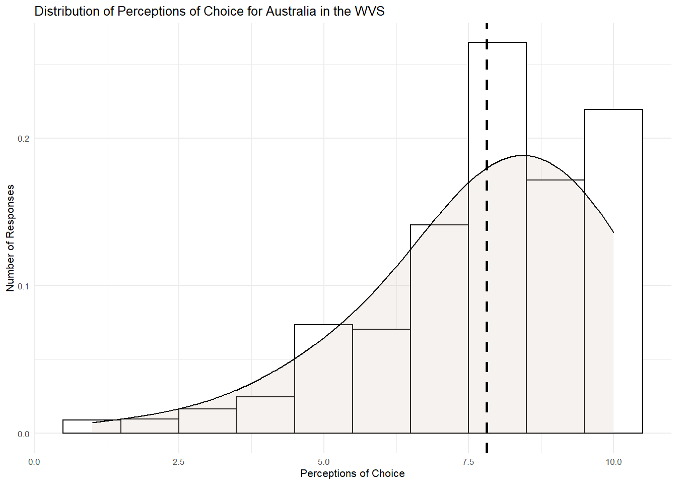
Most people do not score 7.81. Some score higher, some score lower. There is also a negative skew here, with extreme scores on the left-hand tail pulling the mean leftwards.
The beauty of the mean as a model is that this slight skew is accounted for by adding all the responses together and dividing them by the sample. In other words, using the mean as the model ensures the higher and lower scores are perfectly balanced. To see this, lets calculate the second important part of our model - the error (or residual). The error, remember, is the difference of the model (mean) from the observed score.
We can calcualte the error by taking the observed score for choice and subtracting it from the mean score. Lets use the mutate function to do that for the participants in this sample.
WVSaus <-
  WVSaus %>%
  mutate(residual_choice = V55 - mean_choice)
WVSaus
## # A tibble: 1,459 x 4
## V55 V2A mean_choice residual_choice
## <labelled> <chr> <dbl> <labelled>
## 1 9 Australia 7.81 1.1932831
## 2 9 Australia 7.81 1.1932831
## 3 6 Australia 7.81 -1.8067169
## 4 8 Australia 7.81 0.1932831
## 5 2 Australia 7.81 -5.8067169
## 6 9 Australia 7.81 1.1932831
## 7 7 Australia 7.81 -0.8067169
## 8 5 Australia 7.81 -2.8067169
## 9 6 Australia 7.81 -1.8067169
## 10 8 Australia 7.81 0.1932831
## # ... with 1,449 more rowsOr
WVSaus$residual_choice <- WVSaus$V55 - WVSaus$mean_choice
WVSaus
## # A tibble: 1,459 x 4
## V55 V2A mean_choice residual_choice
## <labelled> <chr> <dbl> <labelled>
## 1 9 Australia 7.81 1.1932831
## 2 9 Australia 7.81 1.1932831
## 3 6 Australia 7.81 -1.8067169
## 4 8 Australia 7.81 0.1932831
## 5 2 Australia 7.81 -5.8067169
## 6 9 Australia 7.81 1.1932831
## 7 7 Australia 7.81 -0.8067169
## 8 5 Australia 7.81 -2.8067169
## 9 6 Australia 7.81 -1.8067169
## 10 8 Australia 7.81 0.1932831
## # ... with 1,449 more rowsNow, if we sum the residuals you will see that they will equal zero. This is the key advantage of using the mean as a model in statistics. It balances the values above and below it. Its quite remarkable that this procedure of adding up all the numbers and dividing by the number of participants results in this balancing point.
Let’s check this by using the sum() function to sum the residuals.
sum(WVSaus$residual_choice)## [1] -2.282619e-13Any time you see R return a slightly gibberish value containing “e-”, it means that this is an incredibly small value that, for all intents and purposes, we can interpret as zero. So here we see the value of the mean as a model. It minimizes the error.
Thinking about the mean in this way also helps us think about DATA = MODEL + ERROR in a more specific way. If the mean is the model, each data point can now be thought of as the sum of the model (7.81 in our WVS data) plus its deviation from the model. So 9 can be decomposed into the model part (7.81) and the error from the model (+1.19).
It’s easy to fit the empty model, which is why I am starting us here — it’s just the mean (7.81 in this case). But later in the course, we will will learn to fit more complex models. I am going to teach you a way of fitting models in R that you can use now for fitting the empty model, but that will also work in subsequent weeks for fitting more complex models.
The R function we are going to use is lm(), which stands for “linear model.” Here’s the code we use to fit the empty linear model.
lm(V55 ~ NULL, data = WVSaus)##
## Call:
## lm(formula = V55 ~ NULL, data = WVSaus)
##
## Coefficients:
## (Intercept)
## 7.807Although the output seems a little odd, with words like “Coefficients” and “Intercept,” it does give you back the mean of the distribution (7.81), as expected. We will see in subsequent weeks why the mean is referred to as the intercept, but for now just think about the intercept as the best fitting model. Our “best guess”, so to speak. The word “NULL” is another word for “empty” (as in “empty model.”)
It will be helpful as we go forward to save the results of this linear model in an R object. Here’s code that uses lm() to fit the empty model, then saves the results in an R object called Aus.model
Aus.model <- lm(V55 ~ NULL, data = WVSaus)
Aus.model
##
## Call:
## lm(formula = V55 ~ NULL, data = WVSaus)
##
## Coefficients:
## (Intercept)
## 7.807Using this model we can request a couple of cool outputs that highlight the key properties of DATA = MODEL + ERROR. First lets request the predicted values from this model using the predict() function and add them to the WVSaus dataframe
WVSaus$predicted <- predict(Aus.model) # add to the WVSaus dataframe a new variable called predicted and save the predicted values from the Aus.model
WVSaus
## # A tibble: 1,459 x 5
## V55 V2A mean_choice residual_choice predicted
## <labelled> <chr> <dbl> <labelled> <dbl>
## 1 9 Australia 7.81 1.1932831 7.81
## 2 9 Australia 7.81 1.1932831 7.81
## 3 6 Australia 7.81 -1.8067169 7.81
## 4 8 Australia 7.81 0.1932831 7.81
## 5 2 Australia 7.81 -5.8067169 7.81
## 6 9 Australia 7.81 1.1932831 7.81
## 7 7 Australia 7.81 -0.8067169 7.81
## 8 5 Australia 7.81 -2.8067169 7.81
## 9 6 Australia 7.81 -1.8067169 7.81
## 10 8 Australia 7.81 0.1932831 7.81
## # ... with 1,449 more rowsNotice that the predicted values from the model are the same as the mean that we calculated? Thats because the model we tested is empty and therefore the mean is the best guess or predicted value!
Great so we have the predicted values from the empty model, lets also use the model to calculate the residuals.
WVSaus$residuals <- resid(Aus.model) # add to the WVSaus dataframe a new variable called residuals and save the residual values from the Aus.model
WVSaus
## # A tibble: 1,459 x 6
## V55 V2A mean_choice residual_choice predicted residuals
## <labelled> <chr> <dbl> <labelled> <dbl> <labelled>
## 1 9 Australia 7.81 1.1932831 7.81 1.1932831
## 2 9 Australia 7.81 1.1932831 7.81 1.1932831
## 3 6 Australia 7.81 -1.8067169 7.81 -1.8067169
## 4 8 Australia 7.81 0.1932831 7.81 0.1932831
## 5 2 Australia 7.81 -5.8067169 7.81 -5.8067169
## 6 9 Australia 7.81 1.1932831 7.81 1.1932831
## 7 7 Australia 7.81 -0.8067169 7.81 -0.8067169
## 8 5 Australia 7.81 -2.8067169 7.81 -2.8067169
## 9 6 Australia 7.81 -1.8067169 7.81 -1.8067169
## 10 8 Australia 7.81 0.1932831 7.81 0.1932831
## # ... with 1,449 more rowsAgain, this output is exactly the same as we calculated by hand. This is no coincidence, the model is subtracting the mean from the observed data and saving it as the residual or error.
Error
Back to the model and lets hone in on the error. Remember when we summed the residuals and were left with a zero value? This highlights the usefulness of the mean in balancing the residuals, but we are left with the problem that the sum of the residuals does not tell us a great deal about the TOTAL amount of error in our model. When the mean is the model, ALL distributions will have a sum of residual equaling zero irrespective of whether the amount of error is large or small. Can you think how we remedy this?
Thats right, we can square the residuals to get rid of the minus values. The sum of squares also has another useful property in that it is minimised at the mean. And this is what we are attempting to do with statistics - minimise the error!
Let’s now square the residuals in our data and save a new variable that contains the squared values.
WVSaus$residuals_square <- WVSaus$residuals^2
WVSaus
## # A tibble: 1,459 x 7
## V55 V2A mean_choice residual_choice predicted residuals residuals_square
## <labe> <chr> <dbl> <labelled> <dbl> <labelle> <labelled>
## 1 9 Aust~ 7.81 1.1932831 7.81 1.19328~ 1.42392449
## 2 9 Aust~ 7.81 1.1932831 7.81 1.19328~ 1.42392449
## 3 6 Aust~ 7.81 -1.8067169 7.81 -1.80671~ 3.26422606
## 4 8 Aust~ 7.81 0.1932831 7.81 0.19328~ 0.03735835
## 5 2 Aust~ 7.81 -5.8067169 7.81 -5.80671~ 33.71796150
## 6 9 Aust~ 7.81 1.1932831 7.81 1.19328~ 1.42392449
## 7 7 Aust~ 7.81 -0.8067169 7.81 -0.80671~ 0.65079220
## 8 5 Aust~ 7.81 -2.8067169 7.81 -2.80671~ 7.87765992
## 9 6 Aust~ 7.81 -1.8067169 7.81 -1.80671~ 3.26422606
## 10 8 Aust~ 7.81 0.1932831 7.81 0.19328~ 0.03735835
## # ... with 1,449 more rowsYou will see that this function has now saved the square of the residuals for each data point. From here, it is easy to calculate the sum of squares for our model. That is, the total amount of error in the model. We just use the sum() function to aggregate the squared residual scores.
sum(WVSaus$residuals_square)## [1] 5373.494We can also check this using a function called anova() to look at the error from the Aus.model lm() object we created earlier. ANOVA stands for ANalysis Of VAriance. Analysis means “to break down”, and in the coming weeks we will use this function to break down the variation of outcome variables into parts. However for now we will use anova() just to test out how much error there is around the model, measured in sum of squares.
anova(Aus.model)## Analysis of Variance Table
##
## Response: V55
## Df Sum Sq Mean Sq F value Pr(>F)
## Residuals 1458 5373.5 3.6855Look at the Sum Sq column and you will see the same value from our calculations above - 5373.5. Woah! Thats a really large number, there must be loads of error in this model right? Well, maybe but also maybe not. You see, the sum of squares for the model is very sensitive to sample size. If the sample size is large then the sum of squares will be large - irrespective of the amount of error. This is because the sum of squares adds together all the squared differences. With a sample size of 1,459, that is almost 1500 squared differences to aggregate. Hence, we have a large number for the sum of squares.
This problem is solved by variance and standard deviation. To calculate variance, we start with sum of squares and then divide by the degress of freedom to end up with a measure of average error around the mean. In other words, the average of the squared deviations. Lets calcualte the variances using R as a simple calculator
5373.5/1458 # the df is N-1. In this case there are 1459 participants in the Australia data, so 1459-1 = 1458. ## [1] 3.685528You will see this value is the same as the Mean Sq value from the ANOVA output. This is becuase these values represent the same thing. Whenever you see Mean Sq you now know it means variance.
Because it is an average, variance is not impacted by sample size, and thus, can be used to compare the amount of error across two samples of different sizes.
We can also express error in terms of standard deviation. The standard deviation is simply the square root of the variance. We generally prefer thinking about error in terms of standard deviation because it yields a number that makes sense using the original scale of measurement. So, for example, if you were modeling responses on a 7-point likert scale, variance would express the error in squared points (not something we are used to thinking about), whereas standard deviation would express the error in original units (i.e., the 7-point scale). Lets again use R as a calculator to work out the SD using the sqrt() function:
sqrt(3.69)## [1] 1.920937We can check this against the output using the favstats() function.
favstats(~V55, data = WVSaus)## min Q1 median Q3 max mean sd n missing
## 1 7 8 9 10 7.806717 1.919772 1459 0These are the same values (1.92) within errors of rounding.
Z Scores
We have looked at the mean as a model and we have learned some ways to quantify total error around the mean, as well as some good reasons for doing so. But there is another reason to look at both mean and error together. Sometimes by putting the two ideas together it can give us a better way of understanding where a particular score falls in a distribution.
Let’s say an Australian participant - Jericho - in the WVS has a perception of choice score at one unit below the mid-point; 6. What does this mean? Does this participant have a particularly high or particularly low score? How can we know? By now you may be getting the idea that just knowing the score of one person doesn’t tell you very much.
To interpret the meaning of Jericho’s single score, it helps to know something about the distribution the score came from.
Standard deviation is really useful here. We know that Jericho’s score is about 2 points lower than the average Australian choice score. But now we also know that, on average, choice scores are 1.9 points away from the mean the SD, both above and below. Although Jericho’s score is below average, it is definitely not one of the lowest in the distribution. Let’s draw another histogram but this time add a layer to it that plots Jericho’s score in the distribution of values.
WVSaus %>%
  ggplot(aes(x= V55)) +
  geom_histogram(aes(y=..density..), binwidth=1, colour="black", fill="white") +
  geom_vline(aes(xintercept=mean(V55)), col="blue", size=1) +
  geom_vline(aes(xintercept=6), col = "red", size=1) +
  ylab("Number of Responses") + # this adds a vertical line for the score of "6"
  xlab("Perceptions of Choice") +
  ggtitle("Distribution of Perceptions of Choice for Australia in the WVS with Blue Line Showing the Mean and Red Line Showing Jericho") +
  theme_minimal(base_size = 8)
## Don't know how to automatically pick scale for object of type labelled. Defaulting to continuous.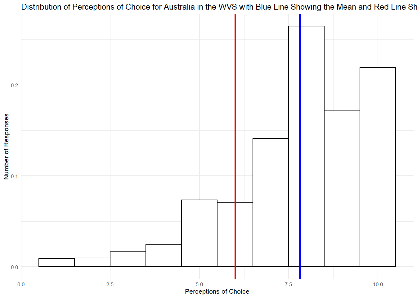
We can combine information from our model regarding the mean and standard deviation to calculate a Z-Score. A single z score tells us how many standard deviations away this particular score of 6 is from the mean. It is calculated by taking any given residual and dividing it by the standard deviation in the sample. We can create Z-scores in our dataframe in two ways. First, we can calcuate it by hand:
WVSaus$Z1 <- WVSaus$residuals/1.92 # remeber the Z score is the residual divided by the SD, in this case 1.92
WVSaus
## # A tibble: 1,459 x 8
## V55 V2A mean_choice residual_choice predicted residuals residuals_square
## <lab> <chr> <dbl> <labelled> <dbl> <labelle> <labelled>
## 1 9 Aust~ 7.81 1.1932831 7.81 1.19328~ 1.42392449
## 2 9 Aust~ 7.81 1.1932831 7.81 1.19328~ 1.42392449
## 3 6 Aust~ 7.81 -1.8067169 7.81 -1.80671~ 3.26422606
## 4 8 Aust~ 7.81 0.1932831 7.81 0.19328~ 0.03735835
## 5 2 Aust~ 7.81 -5.8067169 7.81 -5.80671~ 33.71796150
## 6 9 Aust~ 7.81 1.1932831 7.81 1.19328~ 1.42392449
## 7 7 Aust~ 7.81 -0.8067169 7.81 -0.80671~ 0.65079220
## 8 5 Aust~ 7.81 -2.8067169 7.81 -2.80671~ 7.87765992
## 9 6 Aust~ 7.81 -1.8067169 7.81 -1.80671~ 3.26422606
## 10 8 Aust~ 7.81 0.1932831 7.81 0.19328~ 0.03735835
## # ... with 1,449 more rows, and 1 more variable: Z1 <labelled>R can also directly calculate Z scores using the scale() function:
WVSaus$Z2 <- scale(WVSaus$V55)
WVSaus
## # A tibble: 1,459 x 9
## V55 V2A mean_choice residual_choice predicted residuals residuals_square
## <lab> <chr> <dbl> <labelled> <dbl> <labelle> <labelled>
## 1 9 Aust~ 7.81 1.1932831 7.81 1.19328~ 1.42392449
## 2 9 Aust~ 7.81 1.1932831 7.81 1.19328~ 1.42392449
## 3 6 Aust~ 7.81 -1.8067169 7.81 -1.80671~ 3.26422606
## 4 8 Aust~ 7.81 0.1932831 7.81 0.19328~ 0.03735835
## 5 2 Aust~ 7.81 -5.8067169 7.81 -5.80671~ 33.71796150
## 6 9 Aust~ 7.81 1.1932831 7.81 1.19328~ 1.42392449
## 7 7 Aust~ 7.81 -0.8067169 7.81 -0.80671~ 0.65079220
## 8 5 Aust~ 7.81 -2.8067169 7.81 -2.80671~ 7.87765992
## 9 6 Aust~ 7.81 -1.8067169 7.81 -1.80671~ 3.26422606
## 10 8 Aust~ 7.81 0.1932831 7.81 0.19328~ 0.03735835
## # ... with 1,449 more rows, and 2 more variables: Z1 <labelled>, Z2[,1] <dbl>You will see that both Z scores are more or less the same, however, it is best to use the scale() function as calculations by hand are liable to minor errors of rounding.
Lets check out the distribution of Z scores using the favstats() function:
favstats(~Z2, data = WVSaus)## min Q1 median Q3 max mean sd n missing
## -3.545586 -0.420215 0.1006802 0.6215754 1.142471 -6.699944e-17 1 1459 0The Z Score has transformed the choice variable so that it now has a mean of zero and a SD of 1. A z score, then, tells you how many standard deviations a score is from the mean of its distribution. Going back to Jericho, if we wanted to calculate his Z score then we just plug in his residual to the Z score calculation:
-1.81/1.92 # Jericho scored 6 and the mean is 7.81 so 6 - 7.81 = -1.81. We take this residual and divide it by the SD of 1.92.## [1] -0.9427083Here we can see that Jericho’s score is almost 1 standard deviation below the Australian mean. If we plot this in a histogram as we did before, but this time with Z scores plotting the error distribution, we can see a similar picture:
WVSaus %>%
  ggplot(aes(x= Z2)) +
  geom_histogram(aes(y=..density..), binwidth=.6, colour="black", fill="white") +
  geom_vline(aes(xintercept=mean(Z2)), col="blue", size=1) +
  geom_vline(aes(xintercept=-.94), col = "red", size=1) +
  ylab("Number of Responses") +
  xlab("Perceptions of Choice") +
  ggtitle("Distribution of Perceptions of Choice Z Scores for Australia in the WVS with Blue Line Showing the Mean and Red Line Showing Jericho") +
  theme_minimal(base_size = 8)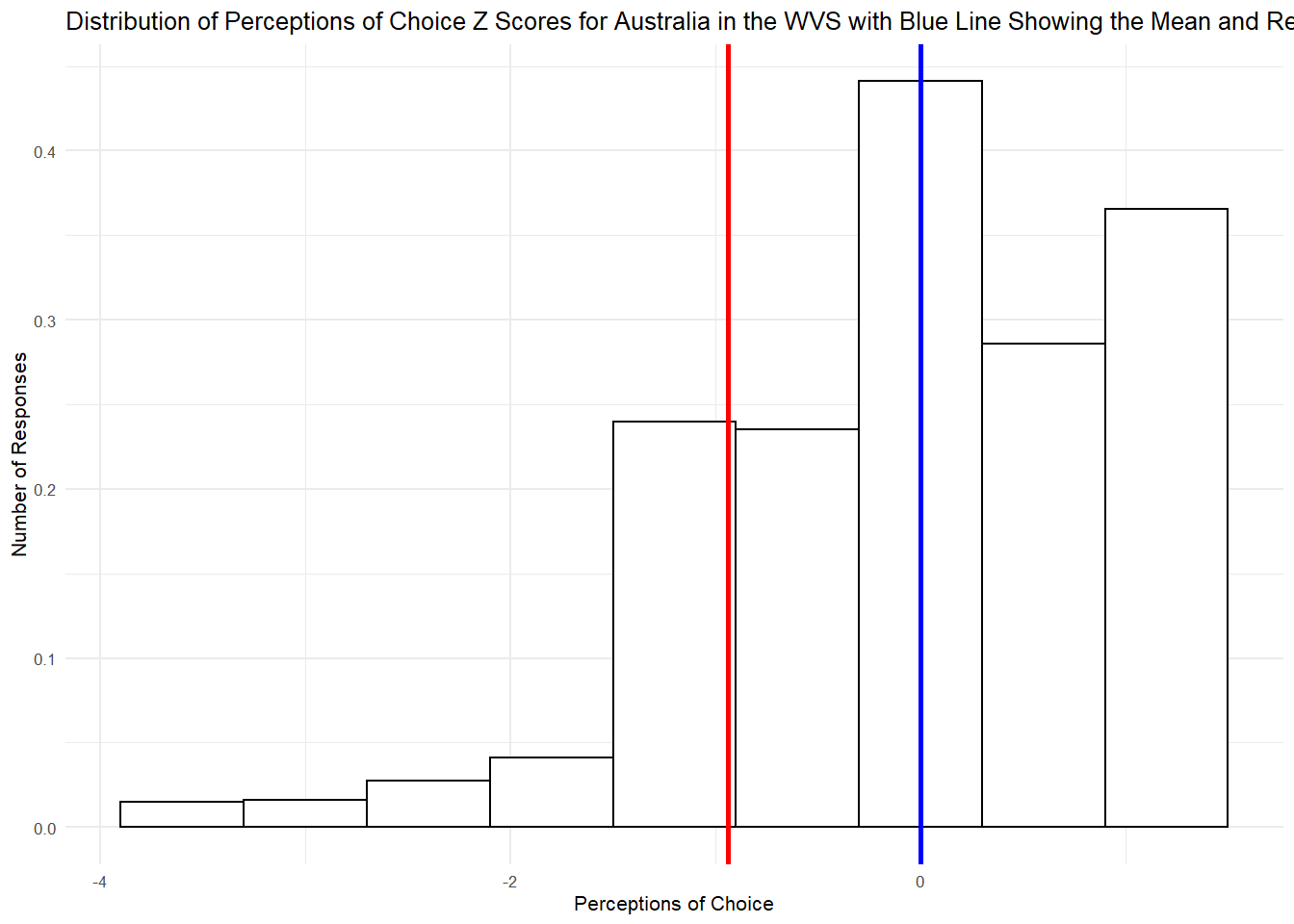
Now with this distribution of Z scores we can do something pretty cool. We can find the normal curve that best fits the data and that normal curve can then be used to make predictions about how likely it is that any randomly sampled Australian would report a perception of choice that is larger than Jericho’s of 6. To do this, we are going to us the xpnorm() function to fit the normal curve and then use it to tell us the exact probability
xpnorm(6, mean = 7.81, sd = 1.92) # 6 is the score we are making predictions about, the mean for the Australia distribution is 7.81 and the SD is 1.92## ## If X ~ N(7.81, 1.92), then## P(X <= 6) = P(Z <= -0.9427) = 0.1729## P(X > 6) = P(Z > -0.9427) = 0.8271## 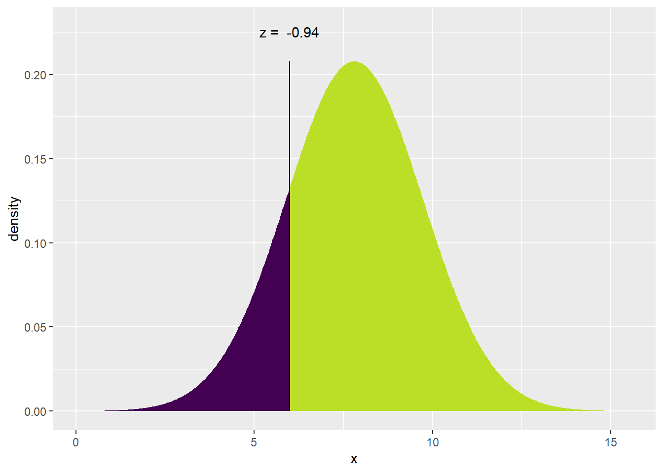
## [1] 0.1729151The first window tells us that there is a 17% chance that any randomly sampled Australian would score less than 6 on perceptions of choice, whereas 83% would report a larger score. Perhaps Jericho is a low scorer after all!
The second window plots Jericho’s score under the fitted normal curve. You can see that his Z-score, -.94, is exactly as we calculated and it cuts off 83% of the sample. Pretty impressive use of our mean and SD!
Activity
Let’s now return to our original aim for this session and imagine that Jericho was Japanese not Australian. Rather than coming from the Australian distribution, his score of 6 came from the Japanese distribution. We know what this score means in Australia but What does it mean in Japan? Does Japanese Jericho have a particularly low score as well? Its your job to find out.
Task 1: Creating the dataframe
First go back to the WVSchoice dataframe we created and filter for usable responses and Japan and save the filtered data as a new dataframe called WVSjapan
WVSjapan <-
  WVSchoice %>%
Task 2: Building the empty model
Now build the empty model by first creating a new variable for the predicted scores. Remeber that in an empty model the predicted or best guess score is the mean:
WVSjapan$predicted <-
WVSjapan
What is the mean score for Japan?
Now create a new variable for the residuals (error):
WVSjapan$residuals <-
WVSjapan
Now create a new variable for residuals squared:
WVS$residuals_squared <-Calcualate the sum of squares for the Japan model:
What is the sum of squares?
Calcualte the variance, remember to use the degrees of freedom in this calculation:
What is the variance?
Calcualte the standard deviation:
What is the standard deviation?
Let’s build the empty model for Japan using the lm() funtion and save it as an R object Japan.model:
Japan.model <- lm() # enter the NULL model you are buildingNow lets check our calculations for the mean and variance using the anova() function:
anova() # enter the name of the model you have built using lm()
anova
Finally, lets check the standard deviation using the favstats () function:
Task 3: Z-scores and prediction
Create a new variable in the WVSjapan dataframe that contains the Z-scores. Remeber to use the scale() function so that we do not run into rounding errors:
WVSjapan$Z <-
WVSjapan
Use the Z-score equation to calcualte the Z score for a Jericho’s value of 6. Remeber the equation is - residual/SD so first find the residual for 6 and then divide it by the standard deviation:
How many standard deviations is Jericho’s score of 6 away from the mean in the Japan distribution?
Now plot the distribution of z scores and add a blue line to represent the mean and a red line to represent Jericho’s score:
Finally, use the xpnorm() function to fit the normal curve around this distribution and find how likely it is that any randomly sampled Japanese person would report a perception of choice that is larger than Jericho’s of 6.
What is the percentage chance that any randomly sampled Japanese person would score less than 6 on perceptions of choice?
What is the percentage chance that any randomly sampled Japanese person would score more than 6 on perceptions of choice?
How does this compare to Australia?