Comparing Groups (MT9)
This week we will move on from the empty model to add categorical explanatory variables that might help to reduce the error or imprecision of statistical estimation. Let’s say we have an empty model that contained 100 student scores of narcissism. Without any other information, our best guess of what any given student might score on narcissism is the mean (i.e., the empty model). However, let’s say we speculate that we might be able to improve our best guess, or reduce our estimated variance, if we knew the gender of the student because males typically score higher on narcissism than females. This is, in essence, what we are doing by adding a categorical explanatory variable to our empty model – attempting to improve the accuracy of our best guess by adding variables that explain the error variation in the empty model.
Learning outcomes
At the end of today’s workshop you should be able to do the following:
Conduct a one-parameter linear model (paired samples t-test) using the lm and t.test functions
Conduct a two-parameter linear model (independent samples t-test) using the lm and t.test model functions
Conduct a three-parameter model (between groups one-way ANOVA) using the lm and aov functions
Load required packages
The required packages are the same as the installed packages. Write the code needed to load the required packages in the below R chunk.
library(mosaic)
library(sjlabelled)
library(fastDummies)
library(supernova)
library(readr)
library(rstatix)
library(Hmisc)
library(ggpubr)
One-parameter linear model or paired samples t-test
To practice conducting a one-parameter linear model with paired differences (paired samples t-test), we are going to use a dataset from Pruzek & Helmreich (2009). This dataset presents 15 paired data corresponding to the weights (lbs) of girls before and after 14-weeks of psychological therapy for anorexia.
The data are from an intervention study with pre and post weights and give a good example of a paired design. Many interventions are set up like this in psychology, and the one-parameter linear model is how we test for differences from pre-test to post-test.
We are going to go through testing these models with the lm() function first, and I’ll then show you the equivalence with the t.test() function.
First, lets load this data into our R environment. Go to the MT9 folder, and then to the workshop folder, and find the “anorexia.csv” file. Click on it aand then select “import dataset”. In the new window that appears, click “update” and then when the dataframe shows, click import. If you want, you can try running the code below and it should do the same thing (if not put your hand up).
anorexia <- read_csv("C:/Users/CURRANT/Dropbox/Work/LSE/PB130/MT9/Workshop/anorexia.csv")## Rows: 15 Columns: 3## -- Column specification --------------------------------------------------------
## Delimiter: ","
## chr (1): Subject
## dbl (2): X1, Y1##
## i Use `spec()` to retrieve the full column specification for this data.
## i Specify the column types or set `show_col_types = FALSE` to quiet this message.anorexia## # A tibble: 15 x 3
## X1 Y1 Subject
## <dbl> <dbl> <chr>
## 1 8.88 10.1 S01
## 2 14.4 11.9 S02
## 3 8.02 6.02 S03
## 4 5.84 3.04 S04
## 5 5.47 1.87 S05
## 6 12.1 12.6 S06
## 7 11.7 9.66 S07
## 8 10.3 9.26 S08
## 9 5.07 6.16 S09
## 10 8.24 10.8 S10
## 11 15.1 12.4 S11
## 12 13.5 10.2 S12
## 13 11.3 12.4 S13
## 14 9.82 9.66 S14
## 15 9.56 6.96 S15You will see that this dataframe has three columns and 15 subjects (rows). X1 is the girls’ pre-therapy weight and Y1 is the girls’ post-therapy weight. The Subject variable is the subject code for each participant.
Before we delve into this topic lets just clarify the research question and null hypothesis we are testing:
Research Question - Do girls have different before and after therapy weights?
Null Hypothesis - The difference between girls’ weight before and after therapy will be zero.
Descriptives
Lets first inspect this data and take a look at the means and standard deviations for each time point. By now, you should know how to do this. As a reminder, we can use favstats() to inspect the descriptives.
favstats(~X1, data=anorexia)## min Q1 median Q3 max mean sd n missing
## 5.065 8.125 9.82 11.89 15.08 9.948667 3.126275 15 0favstats(~Y1, data=anorexia)## min Q1 median Q3 max mean sd n missing
## 1.87 6.555 9.66 11.3625 12.64 8.87 3.365538 15 0Okay, there appears to be a small reduction in weight from pre to post therapy evidenced by the means (not a good start). But there is quite substantial variance in both samples, as evidenced by the SD, so the question is whether this mean difference is statistically meaningful. Is it large enough for us to conclude that a zero effect is unlikely?
To address this question, lets first calculate the difference scores for each participant and take a look at the mean difference between the pairs.
anorexia$difference <- anorexia$Y1 - anorexia$X1
anorexia
## # A tibble: 15 x 4
## X1 Y1 Subject difference
## <dbl> <dbl> <chr> <dbl>
## 1 8.88 10.1 S01 1.25
## 2 14.4 11.9 S02 -2.44
## 3 8.02 6.02 S03 -1.99
## 4 5.84 3.04 S04 -2.79
## 5 5.47 1.87 S05 -3.6
## 6 12.1 12.6 S06 0.58
## 7 11.7 9.66 S07 -2.06
## 8 10.3 9.26 S08 -1.05
## 9 5.07 6.16 S09 1.09
## 10 8.24 10.8 S10 2.55
## 11 15.1 12.4 S11 -2.72
## 12 13.5 10.2 S12 -3.31
## 13 11.3 12.4 S13 1.08
## 14 9.82 9.66 S14 -0.160
## 15 9.56 6.96 S15 -2.61Lets now use favstats again to examine the mean difference between the paired scores.
favstats(~difference, data=anorexia)## min Q1 median Q3 max mean sd n missing
## -3.6 -2.665 -1.99 0.83 2.55 -1.078667 1.973018 15 0Here we have a mean reduction of 1.08 lbs from before to after therapy. The SD associated with that reduction is 1.97. We can also think about this mean difference as our predicted value, like the mean was the predicted value in the empty model. All else being equal and with no other information, our best guess would be that the psychological therapy would result in a weight reduction of 1.08 lbs. As we saw with the descriptives, this is not good news for our intervention.
Setting up the linear model
Okay, lets set our up our linear model to examine the statistical significance of that -1.08 lb mean difference. Like last week, we are using the lm function to test a one-parameter model - but this time the parameter is the difference between the pairs of observations.
anorexia.model <- lm(Y1 - X1 ~ NULL, data=anorexia) # notice how I've set this up. The lm is taking the difference score (Y1- X1) and inputting it to a one-parameter model (NULL). I am then saving that model as an R object called anorexia.model
summary(anorexia.model) # the summary command just calls the summary statistics for the anorexia.model
##
## Call:
## lm(formula = Y1 - X1 ~ NULL, data = anorexia)
##
## Residuals:
## Min 1Q Median 3Q Max
## -2.5213 -1.5863 -0.9113 1.9087 3.6287
##
## Coefficients:
## Estimate Std. Error t value Pr(>|t|)
## (Intercept) -1.0787 0.5094 -2.117 0.0526 .
## ---
## Signif. codes: 0 '***' 0.001 '**' 0.01 '*' 0.05 '.' 0.1 ' ' 1
##
## Residual standard error: 1.973 on 14 degrees of freedomNotice that the model part of this formula - bo - is the same as the mean difference we just calculated -1.08 lbs? This shows that we still have a one-parameter model here but instead of the mean of an outcome in the empty model, this time we have the mean of the differences in the outcome variable for our paired t-test.
Notice also we have some other statistics that we didn’t see in the empty model. The standard error is the estimate of error in the estimate of the model due to sampling variance. It is calculated by taking the standard deviation of the mean difference and dividing it by the sqrt of the sample size. Larger sample sizes and smaller mean difference deviations result in a smaller standard error of the estimate. We calculate this by hand using the information we have already called.
1.973018/sqrt(15) # 1.97 is the SD for the mean difference and the sample size is 15## [1] 0.5094311We also have a t-ratio. This is the ratio of the model estimate - bo - to its standard error. The larger the estimate relative to the SE the larger t will be. Here we have a t-ratio of -2.117. We can also calculate this by hand using the information we have already called.
-1.0787/0.5094311 # ratio of the estimate (mean difference) to the standard error## [1] -2.11746So we have a t-ratio for the mean difference between the pre and post-therapy weights of -2.12. But is this large enough to be statistically significant? Can we say that a zero mean difference is unlikely given the data?
Well take a look at the p value (pr) in the lm () output and remember we said that statisticians count .05 and lower probabilities as unlikely. Our p value is > .05 and therefore we cannot reject the null hypothesis. It seems that weight appears to fall across the time periods in our sample but that decrease is not statistically significant.
We might write this up in a research paper as follows:
There was no statistically significant difference between pre-therapy and post-therapy weight in the current sample: t(14) = -2.12, p > .05.
Equivalence with the paried t.test
Just to show you that the paired t-test is equivalent to a linear model, lets do the same analysis using the t.test function.
t.test(anorexia$Y1, anorexia$X1, paired = TRUE) # setting up the t-test requires the post then pre variables entered in order rathern than as a difference score - R calcualtes the difference score for us in the t.test function.##
## Paired t-test
##
## data: anorexia$Y1 and anorexia$X1
## t = -2.1174, df = 14, p-value = 0.05261
## alternative hypothesis: true difference in means is not equal to 0
## 95 percent confidence interval:
## -2.17128734 0.01395401
## sample estimates:
## mean of the differences
## -1.078667See how the t ratio, p-value and mean difference is exactly the same as the linear model we tested? Thats because the analyses are exactly the same! Students are often taught paired t-test as a separate statistical test to independent t-test, ANOVA and regression (these are tests we will come onto here and in subsequent weeks) but, in fact, they are all a family of tests belonging to the linear model. This equivalence helps us understand what is happening when we run stats in the psychological and behavioral sciences. Its all underpinned by the linear model.
Plotting the paired sample t-test
We might plot this difference using side-by-side boxplots like we did in the visualization week (MT4). Here is the code to place the distributions of the two time points side-on using ggplot.
library(rstatix)
library(ggpubr)
# Transform into long data:
# gather the before and after values in the same column
anorexia.long <- anorexia %>%
  tidyr::gather(key = "Time", value = "weight", X1, Y1)

# create box-plots
bxp <- ggpubr::ggpaired(anorexia.long, x = "Time", y = "weight",
         order = c("X1", "Y1"),
         ylab = "Weight", xlab = "Time")

# Add p-value and significance levels
stat.test <- anorexia.long  %>%
  t_test(weight ~ Time, paired = TRUE) %>%
  add_significance()
stat.test <- stat.test %>% add_xy_position(x = "Time")
bxp + stat_pvalue_manual(stat.test, tip.length = 0) +
  labs(subtitle = get_test_label(stat.test, detailed= TRUE))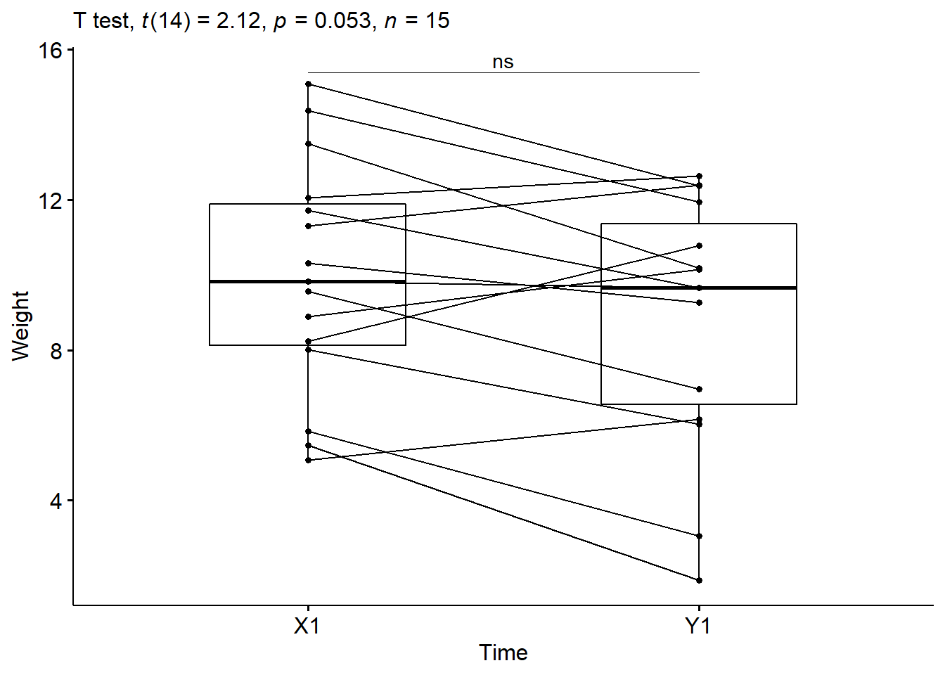
How it’s written
We could report the result as follows:
The mean pre-intervention weight was 9.95 lbs (SD = 3.13), whereas the mean post-intervention weight was 8.87 lbs(SD = 3.37). A paired-sample t-test showed that the difference was not statistically significant, mean diff = -1.08 lbs, t(14) = -2.12, p > 0.05.
Two-parameter model or independent t-test
Okay lets now move to a different research topic and question to examine differences between independent groups. We will start with a two-parameter model (two groups) and move to a three parameter model. As we saw in the lecture, the two-parameter model is often called an independent t-test and the three-parameter model is often called ANOVA. Like the paired t-test, we will see that both of these tests are linear models that can be analyzed using the lm() in R.
To start, lets ask different research question using some data I have collected on levels of perfectionism in American, Canadian, and British college students. This data is from Curran & Hill (2019). Many observational studies in psychology are set up like this, and the two-parameter linear model is how we test for differences in scores across the countries.
Lets start by collapsing the USA and Canada into one region called North America and look to see if North American students differ in their levels of perfectionism to those in the UK. Later, we will extend this model to look at differences across the three counties.
First, lets load this data into our R environment. Go to the MT9 folder, and then to the workshop folder, and find the “perfectionism.csv” file. Click on it and then select “import dataset”. In the new window that appears, click “update” and then when the dataframe shows, click import. If you want, you can run the code below and it will do the same thing.
library(readr)
perfectionism <- read_csv("C:/Users/CURRANT/Dropbox/Work/LSE/PB130/MT9/Workshop/perfectionism.csv")
## Rows: 139 Columns: 4## -- Column specification --------------------------------------------------------
## Delimiter: ","
## chr (3): Study, Country, Region
## dbl (1): SOP##
## i Use `spec()` to retrieve the full column specification for this data.
## i Specify the column types or set `show_col_types = FALSE` to quiet this message.perfectionism## # A tibble: 139 x 4
## Study SOP Country Region
## <chr> <dbl> <chr> <chr>
## 1 Hewitt & Flett 4.39 CAN NORTH_AMERICA
## 2 Hewitt & Flett 4.53 CAN NORTH_AMERICA
## 3 Hewitt & Flett 4.45 CAN NORTH_AMERICA
## 4 Westra TH 4.64 CAN NORTH_AMERICA
## 5 Flett 4.57 CAN NORTH_AMERICA
## 6 Flett 4.56 CAN NORTH_AMERICA
## 7 Flett 4.53 CAN NORTH_AMERICA
## 8 Flett 4.67 CAN NORTH_AMERICA
## 9 Hart et al 4.92 UK UK
## 10 Bottos & Dewey 4.81 CAN NORTH_AMERICA
## # ... with 129 more rowsYou will see that this dataframe has four columns and 139 data points (rows). Study is the study that the mean level of perfectionism was taken from, SOP is the mean level of self-oriented perfectionism reported in the study, Country is the varaible containing the country that the data was collected in (i.e., Canada, the USA, and the UK), and Region (i.e., North America and the UK) is the World region that the data was collected from.
Before we delve into this topic lets just clarify the research question for our two-parameter model and null hypothesis we are testing:
Research Question - Do levels of perfectionism differ between college students from North America and the UK?
Null Hypothesis - The difference between college students’ levels of perfectionism in North America and the UK will be zero.
Descriptives
Lets first inspect this data and take a look at the means and standard devations for each region. By now, you should know how to do this. As a reminder, we can use favstats() to inpect the descriptives.
favstats(~SOP, Region, data=perfectionism) # the second line of fav stats is our factor and it splits the SOP scores into a mean for North America and a mean for the UK.## Region min Q1 median Q3 max mean sd n
## 1 NORTH_AMERICA 4.140000 4.480000 4.595333 4.7190 5.22 4.607002 0.1861641 115
## 2 UK 3.576667 4.335333 4.584333 4.7445 5.21 4.513348 0.3505012 24
## missing
## 1 0
## 2 0Okay, there appears to be a small difference here and we can calculate this difference by hand. We just take the UK mean from the North America mean to ascertain the increment needed from the UK to get the North America mean.
4.607002 - 4.513348## [1] 0.093654North American students appear to have a higher scores on perfectionism than UK students. The difference is 0.093654 points on a 1-7 Likert scale, which doesnt seem a great deal but in the context of the equally small SD, could be significant. The question therefore is whether this mean difference is statistically meaningful or large enough for us to consider the possibility of a zero difference in the population unlikely.
Setting up the linear model
Now lets set our up our linear model to examine the statitical significance of that 0.09 mean difference. This time though we are using the lm() function to test a two-parameter linear model becuase we now have two means to estimate.
Before we do so, I want to show you how to dummy code the variables because the meaning of the intercept changes in line with how the explanatory variable is coded. The intercept, remember, is the value of the outcome (perfectionism) when the explanatory variable equals zero. And so the meaning of zero becomes very important. In this example, I want to know what the increment is from the UK mean to the North America mean, so I’m going to dummy code my explanatory variable as UK = 0 and North America = 1. This way, the interpretation of b0 (intercept) is the UK mean, and the interpretation of b1 is the increment needed for the North America mean or - in other words - the mean difference. To do so, I’m just going use the ifelse() function to assign codes.
perfectionism$dummy <- ifelse(perfectionism$Region == c("NORTH_AMERICA"), 1, 0) # this code creates new variable "dummy" and inserts either 1 or 0 depending on whether North America is TRUE in the Region variable
perfectionism
## # A tibble: 139 x 5
## Study SOP Country Region dummy
## <chr> <dbl> <chr> <chr> <dbl>
## 1 Hewitt & Flett 4.39 CAN NORTH_AMERICA 1
## 2 Hewitt & Flett 4.53 CAN NORTH_AMERICA 1
## 3 Hewitt & Flett 4.45 CAN NORTH_AMERICA 1
## 4 Westra TH 4.64 CAN NORTH_AMERICA 1
## 5 Flett 4.57 CAN NORTH_AMERICA 1
## 6 Flett 4.56 CAN NORTH_AMERICA 1
## 7 Flett 4.53 CAN NORTH_AMERICA 1
## 8 Flett 4.67 CAN NORTH_AMERICA 1
## 9 Hart et al 4.92 UK UK 0
## 10 Bottos & Dewey 4.81 CAN NORTH_AMERICA 1
## # ... with 129 more rowsNow a new variable is created that assigns UK a code 0 and North America a code 1. In reality, the lm() function in R will do this for you if you feed it a categorical variable, but I wanted to show you how this is working.
Okay lets now build our two-parameter model.
perfectionism.model <- lm(SOP ~ 1 + dummy, data=perfectionism) # notice how I've set this up. Unlike the empty or one-parameter model we now have a variable after the tilda (~). This is no longer an empty model with just the mean or intercept but it now contains an intercept (1) and an explainatory variable - namely, our dummy coded region. Thus y ~ 1 + x is the R-way of writing y = b + mx (the stright line equation!).

summary(perfectionism.model) # the summary command just calls the summary statistics for the perfectionism.model
##
## Call:
## lm(formula = SOP ~ 1 + dummy, data = perfectionism)
##
## Residuals:
## Min 1Q Median 3Q Max
## -0.93668 -0.13667 0.00833 0.13300 0.69665
##
## Coefficients:
## Estimate Std. Error t value Pr(>|t|)
## (Intercept) 4.51335 0.04540 99.417 <2e-16 ***
## dummy 0.09365 0.04991 1.876 0.0627 .
## ---
## Signif. codes: 0 '***' 0.001 '**' 0.01 '*' 0.05 '.' 0.1 ' ' 1
##
## Residual standard error: 0.2224 on 137 degrees of freedom
## Multiple R-squared: 0.02506, Adjusted R-squared: 0.01794
## F-statistic: 3.521 on 1 and 137 DF, p-value: 0.06272Notice that the intercept part of our model - bo - is the same as the mean perfectionism score for the UK - 4.51? Notice also that b1 is the mean difference or the increment needed to get to the North American mean (i.e., 0.09 + 4.51 = 4.60)? This shows that we now have two parameters, and a mean difference that is exactly as we calculated by hand.
Notice also we have the same other statistics as in our previous model. The standard error and the t-ratio. From what you now know about these statistics, you should be able to work out whether the difference of .09 is statistically meaningful. We have a t of 1.88 and a p value of .06 - we cannot reject the null hypothesis.
Partitioning variance
Another, perhaps more informative, way to think about this analysis is that we are adding an explanatory variable to the empty model. By doing this, we are attempting to reducing the empty model error. Or, in other words, to explain or reduce the empty model variance. This is the key to statistics; entering information to models that helps us make better predictions. Our reasoning here is that we can better predict perfectionism scores if we know which region a person comes from.
We’ve established that we cannot be certain that the mean difference in the population is not zero (i.e., p > .05), but how much variance in perfectionism is explained by region? We can answer this question using the supernova() function in R, which breaks down the variance in perfectionism due to the model (ie., Region) and error (i.e., variance left over once we’ve subtracted out the model)
library(supernova)
supernova(perfectionism.model)
## Analysis of Variance Table (Type III SS)
## Model: SOP ~ 1 + dummy
##
## SS df MS F PRE p
## ----- --------------- | ----- --- ----- ----- ------ -----
## Model (error reduced) | 0.174 1 0.174 3.521 0.0251 .0627
## Error (from model) | 6.776 137 0.049
## ----- --------------- | ----- --- ----- ----- ------ -----
## Total (empty model) | 6.951 138 0.050Taking a look at the supernova table tells us that the total variance - or sum of squares - in perfectionism scores is 6.95. This is variance of perfectionism in the empty model (i.e., the mean as the model). Entering our predictor in the model reduced the sum of squares in the empty perfectionism model by 0.17. We have, then, a sum of squares 6.78 left after subtracting out the model that includes our predictor (i.e., 6.95-0.17).
When we look at the ratio of total variance (in the empty model) to error variance (in the one-parameter model) we are left with the proportion of empty model variance explained by the model, or PRE. We can see in this example that the PRE is .03. So only about 3% of perfectionism variance is explained by Region. Not a great deal.
Everytime we add a predictor to the model, we spend a degree of freedom and the RPE does not take this into consideration (because it is calculated using the sum of squares). However, the F ratio does take degrees of freedom into consideration because it is the ratio of model variance (SS/df) to error variance (SS/df). You can think about it like the ratio variance explained in the model to variance unexplained in the model. Because variance is calculated using the degrees of freedom, the F-ratio tells us whether the degrees of freedom that we spent in order to make our model more complicated (i.e., adding a parameter) were “worth it”.
In this case, we see an F ratio of 3.52 and a p value of .06. In line with what you understand about p values, this is not statistically significant. Therefore, the interpretation is that adding region to the empty model was not worth it. The variance explained was too small to justify the additional parameter. Notice that this chimes with the interpretation of the t ratio - that there is no significant difference between the groups.
Equivalence with the independent t.test
Just to show you that the independent t-test is equivalent to a linear model, lets do the same analysis using the t.test function.
t.test(perfectionism$SOP ~ perfectionism$dummy, var.equal=TRUE) # setting up the t-test requires the outcome variance and the explanatory variance separated by tilda (~) - R calcualtes the difference score for us in the t.test function.##
## Two Sample t-test
##
## data: perfectionism$SOP by perfectionism$dummy
## t = -1.8764, df = 137, p-value = 0.06272
## alternative hypothesis: true difference in means is not equal to 0
## 95 percent confidence interval:
## -0.192349245 0.005041167
## sample estimates:
## mean in group 0 mean in group 1
## 4.513348 4.607002See how the t ratio, p-value and mean difference is exactly the same as the linear model we tested? Thats because the analyses are exactly the same! Students are often taught independent t-test as a separate statistical test to paired t-test, ANOVA, and regression but, in fact, they are all a family of tests belonging to the linear model! Its all underpinned by the linear model.
Effect size
The effect size is calculated by dividing the mean difference between the groups by the pooled standard deviation.
Cohen’s d formula:
d = (mean1 - mean2)/pooled.sd, where:
pooled.sd is the common standard deviation of the two groups.
pooled.sd = sqrt([var1(n1-1) + var2(n2-1)]/[n1 + n2 -2]);
var1 and var2 are the variances (squared standard deviation) of group1 and 2, respectively.
n1 and n2 are the sample counts for group 1 and 2, respectively. mean1 and mean2 are the means of each group, respectively.
We can do this by hand. But we can also calculate this directly (and more quickly) using the cohens_d function, which is part of the package rstatix:
perfectionism %>%
cohens_d(SOP ~ Region)
## # A tibble: 1 x 7
## .y. group1 group2 effsize n1 n2 magnitude
## * <chr> <chr> <chr> <dbl> <int> <int> <ord>
## 1 SOP NORTH_AMERICA UK 0.334 115 24 smallAccording to Cohen (1988, 1992), the effect size is low if the value of d varies around 0.2, medium if d varies around 0.5, and large if d varies more than 0.8. An d of .33 is a small effect.
Plotting the independent t-test
We might plot this difference using side-by-side boxplots like we did in the visualization week (MT4). Here is the code to place the distributions of the two categories side-on using ggplot.
perfectionism %>%
ggplot(aes(x= Region, y = SOP)) + # remember to use the category variable and not the dummy variable as x here
  geom_boxplot(width = 0.3, fill = "white") +
  geom_jitter(aes(color = as.factor(Region), shape = as.factor(Region)), width = 0.1, size = 1) +
  xlab(NULL) +
  ggtitle("Box-Plots for Perfectionism in UK and North America") +
  theme_minimal(base_size = 8) +
  theme(legend.title=element_blank())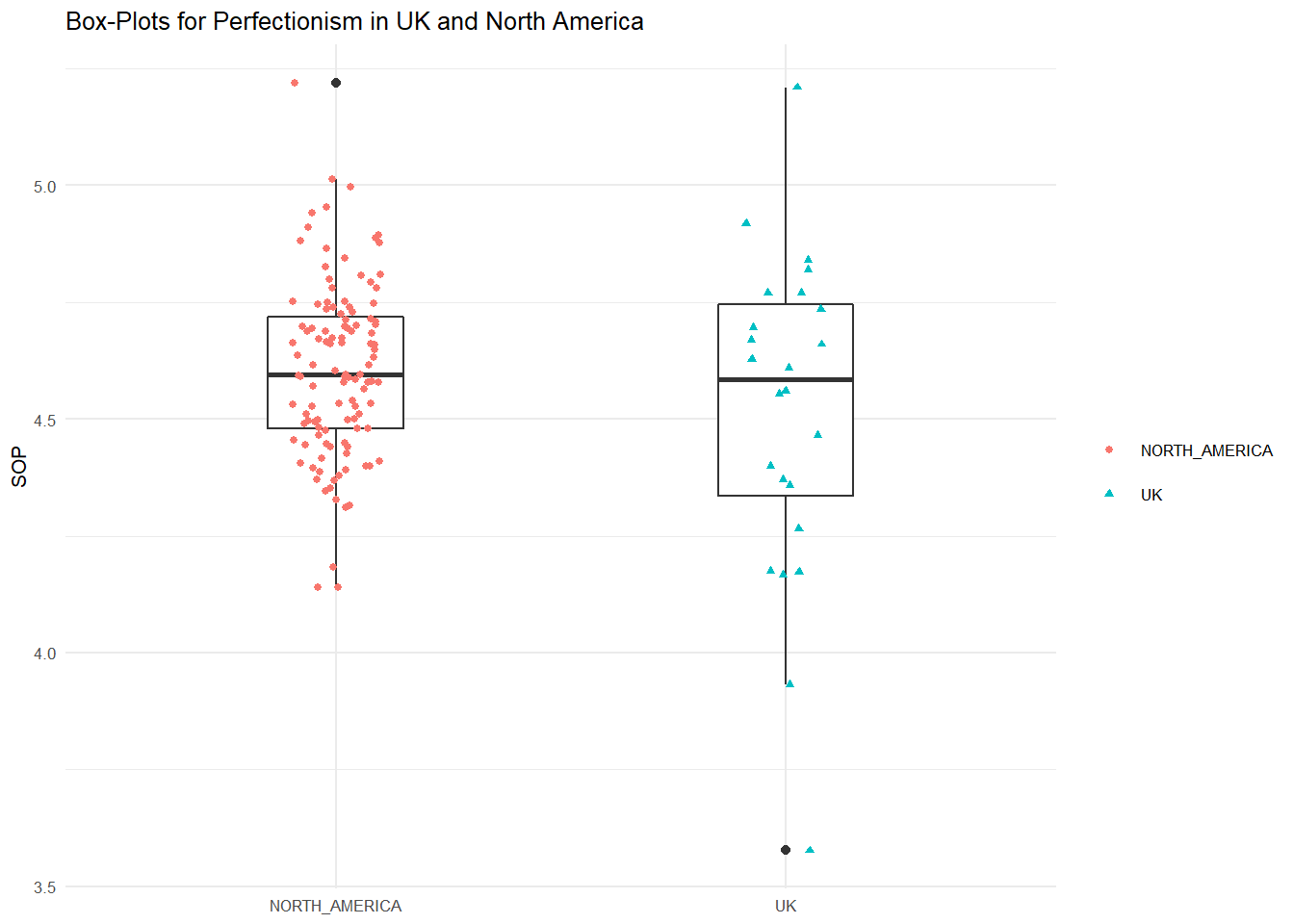
How its written
We could report the result as follow:
The mean perfectionism in UK group was 4.51 (SD = .19), whereas the mean in North America group was 4.61(SD = .35). A two-samples t-test showed that the difference was not statistically significant, t(137) = -1.8764, p > 0.05, d = .33; where, t(137) is shorthand notation for a t-statistic that has 137 degrees of freedom.
Three-parameter model or one-way ANOVA
Lets stay with the perfectionism data but this time we are going to test for difference between USA, Canada, and the UK rather than the UK and North America. Such an analysis, whereby three means are compared is often called a between groups one-way ANOVA in the literature, but we will see it is really just another linear model - this time with three parameters rather than two.
Before we start, lets just clarify the research question for our three-parameter linear model and null hypothesis we are testing:
Research Question - Do levels of perfectionism differ between college students from the USA, Canada, and the UK?
Null Hypothesis - The difference between college students’ levels of perfectionism in the USA, Canada, and UK will be zero.
Descriptives
Lets first inspect this data and take a look at the means and standard devations for each country. By now, you should know how to do this. As a reminder, we can use favstats() to inpect the descriptives.
favstats(~SOP, Country, data=perfectionism) # the second line of fav stats is our factor and it splits the SOP scores into a mean for USA, a mean for Canada, and a mean for the UK.## Country min Q1 median Q3 max mean sd n
## 1 CAN 4.140000 4.446000 4.569333 4.6940 5.220000 4.576998 0.1961644 73
## 2 UK 3.576667 4.335333 4.584333 4.7445 5.210000 4.513348 0.3505012 24
## 3 USA 4.368000 4.578667 4.685216 4.7450 4.997333 4.659151 0.1562029 42
## missing
## 1 0
## 2 0
## 3 0Okay, there appears to be small differences here and we can calculate these differences by hand.
4.576998-4.513348 # CAN-UK diff## [1] 0.063654.576998-4.659151 # CAN-USA diff## [1] -0.0821534.513348-4.659151 # UK-USA diff## [1] -0.145803We can see that Canadians have higher levels of perfectionism than Brits but lower levels than Americans. Americans have higher levels of perfectionism than Brits. Again, the differences are small, but in the context of the small SD these may be significant. The question therefore is whether these mean differences are statistically meaningful.
Setting up the linear model
Now lets set our up our linear model to examine the statitical significance of those mean differences. This time though we are using the lm() function to test a three-parameter model becuase we now have three means to estimate.
Before we do so, like the two-parameter model, I want to show you how to dummy code the variables in a three-group model because the meaning of zero is very important. In this case, we need to create two dummy variables with UK as the reference group. I have chosen UK as the reference group because we know it has the lowest mean (but you can set it up whichever way you want). This necessitates the creation of a USA vs others contrast (USA = 1, others = 0), and a Canada vs others contrast (Canada = 1, others = 0). Setting it up this way makes in the interpretation of the intercept the UK mean (because UK is always coded 0), b1 the increment needed to find the USA mean from the UK mean, and b2 the increment needed to find the Canada mean from the UK mean. The difference between b1 and b2 gives the mean difference between the USA and Canada.
We could code the variables by hand but there is a useful function in R that does this for us. Its called fastdummies and uses a dummy_cols() function to dummy code variables given a categorical input. So lets go ahead and create those dummy variables.
perfectionism <- dummy_cols(perfectionism, select_columns = "Country") # into the perfectionism dataframe create dummy columns using the "Country" variable in the perfectionism data frame
perfectionism
## # A tibble: 139 x 8
## Study SOP Country Region dummy Country_CAN Country_UK Country_USA
## <chr> <dbl> <chr> <chr> <dbl> <int> <int> <int>
## 1 Hewitt & Flett 4.39 CAN NORTH_~ 1 1 0 0
## 2 Hewitt & Flett 4.53 CAN NORTH_~ 1 1 0 0
## 3 Hewitt & Flett 4.45 CAN NORTH_~ 1 1 0 0
## 4 Westra TH 4.64 CAN NORTH_~ 1 1 0 0
## 5 Flett 4.57 CAN NORTH_~ 1 1 0 0
## 6 Flett 4.56 CAN NORTH_~ 1 1 0 0
## 7 Flett 4.53 CAN NORTH_~ 1 1 0 0
## 8 Flett 4.67 CAN NORTH_~ 1 1 0 0
## 9 Hart et al 4.92 UK UK 0 0 1 0
## 10 Bottos & Dewey 4.81 CAN NORTH_~ 1 1 0 0
## # ... with 129 more rowsYou will see that this function returns three new dummy variables - Country_CAN, Country_USA, and Country_UK. This is quite cool because it is giving us the option of which group to use as the reference. I have said we should use the UK as the reference because it has the lowest mean. So the two variables we will carry forward for our analysis are: Country_CAN and Country_USA.
Okay lets now build our three-parameter model.
perfectionism.model2 <- lm(SOP ~ 1 + Country_USA + Country_CAN, data=perfectionism) # notice how I've set this up. Unlike the empty or two-parameter models we now have two variables after the tilda (~). This is no longer an empty model with just the mean or intercept and one additional parameter, but it now contains an intercept (1) and a two explainatory variables - namely, our dummy coded coutries USA and Canada.

summary(perfectionism.model2) # the summary command just calls the summary statistics for the perfectionism.model
##
## Call:
## lm(formula = SOP ~ 1 + Country_USA + Country_CAN, data = perfectionism)
##
## Residuals:
## Min 1Q Median 3Q Max
## -0.93668 -0.13141 0.01367 0.12900 0.69665
##
## Coefficients:
## Estimate Std. Error t value Pr(>|t|)
## (Intercept) 4.51335 0.04496 100.396 <2e-16 ***
## Country_USA 0.14580 0.05635 2.587 0.0107 *
## Country_CAN 0.06365 0.05182 1.228 0.2215
## ---
## Signif. codes: 0 '***' 0.001 '**' 0.01 '*' 0.05 '.' 0.1 ' ' 1
##
## Residual standard error: 0.2202 on 136 degrees of freedom
## Multiple R-squared: 0.05094, Adjusted R-squared: 0.03699
## F-statistic: 3.65 on 2 and 136 DF, p-value: 0.02856Notice that the intercept part of our model - bo - is the same as the mean perfectionism score for the UK - 4.51? Notice also that b1 is the mean difference or the increment needed to get to the USA mean (i.e., 0.15 + 4.51 = 4.66) and b2 is the mean difference or increment needed to get to the Canada mean (i.e., 0.06 + 4.51 = 4.57)? The difference between b1 and b2 (.08) is the mean difference between USA and Canada. This shows that we now have three parameters, and mean differences that are exactly as we calculated by hand.
Notice also we have the same other statistics as in our previous model. The standard error and the t-ratio. From what you now know about these statistics, you should be able to work out whether the difference of .15 between the UK and USA is statistically significant. We have a t of and a p value of .01 - we can reject the null hypothesis. For the UK vs Canada difference of .06 we have a t ratio of 1.228 and a p value of 0.22 - we cannot reject he null hypothesis.
Plotting the one-way ANOVA
We might plot this difference using side-by-side boxplots like we did above. Here is the code to place the distributions of the three categories side-on using ggplot.
perfectionism %>%
ggplot(aes(x= Country, y = SOP)) + # remember to use the category variable and not the dummy variable as x here
  geom_boxplot(width = 0.3, fill = "white") +
  geom_jitter(aes(color = as.factor(Country), shape = as.factor(Country)), width = 0.1, size = 1) +
  xlab(NULL) +
  ggtitle("Box-Plots for Perfectionism in UK, Canada, and USA") +
  theme_minimal(base_size = 8) +
  theme(legend.title=element_blank())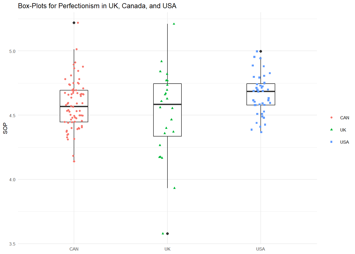
Partitioning variance
As we saw with the two-parameter model, another way to think about this analysis is that we are adding two explainatory variables to the empty model. By doing this, we are attempting to reduce the empty model error. Or, in other words, to explain or reduce the empty model variance. That is the key to statistics; entering information to models that helps us make better predictions. Our reasoning here is that we can better predict perfectionism scores if we know which country a person comes from.
We’ve established that the mean difference in the population is not zero for USA vs UK but not Canada vs UK, but how much variance in perfectionism is explained by country? And is this meaningful? Again, we can answer this question using the supernova() function in R, which breaks down the variance in perfectionism due to the model (ie., country) and error (i.e., variance left over once we’ve subtracted out the model).
supernova(perfectionism.model2)## Analysis of Variance Table (Type III SS)
## Model: SOP ~ 1 + Country_USA + Country_CAN
##
## SS df MS F PRE p
## ----------- --------------- | ----- --- ----- ----- ------ -----
## Model (error reduced) | 0.354 2 0.177 3.650 0.0509 .0286
## Country_USA | 0.325 1 0.325 6.694 0.0469 .0107
## Country_CAN | 0.073 1 0.073 1.509 0.0110 .2215
## Error (from model) | 6.597 136 0.049
## ----------- --------------- | ----- --- ----- ----- ------ -----
## Total (empty model) | 6.951 138 0.050Taking a look at the supernova table tells us that the total variance - or sum of squares - in perfectionism scores is 6.95. This is variance of perfectionism in the empty model (i.e., the mean as the model). Entering our two dummy predictors in the model reduced the sum of squares in the empty perfectionism model by 0.354. We have, then, a sum of squares 6.60 left after subtracting out the model that includes our predictor (i.e., 6.95-0.35). Compare this with the meager 0.17 sum of squares explained by Region - splitting region in two and looking at perfectionism scores across the USA, Canada, and UK has explained far more variance. Why? Well, because Americans have much higher perfectionism scores than Brits and Canadians! In other words, the USA explains error variance in the empty perfectionism model.
When we look at the ratio of total variance (in the empty model) to error variance (in the one-parameter model) we are left with the proportion of empty model variance explained by the model, or PRE. We can see in this example that the PRE is .05. So about 5% of perfectionism variance is explained by Country. Again, compare this to the 3% explained by Region in the two-parameter model.
Remember, though, that adding an additional parameter will always result in some variance explained by chance, so the question becomes - is this increase in explained variance enough given the additional model complexity?
Everytime we add a predictor to the model, we spend a degree of freedom and the RPE does not take this into consideration. However, the F ratio does because it is the ratio of model variance to error variance. Because variance is calculated using the degrees of freedom, the F-ratio tells us whether the degrees of freedom that we spent in order to make our model more complicated (i.e., adding a parameter) as “worth it”.
In this case, we see an F ratio associated with the model of 3.65 and a p value of .03. In line with what you understand about p values, this is a statistically significant result! Therefore, the interpretation is that adding our two Country dummy variables to the empty model was worth it. The variance explained is large enough to justify the additional parameter. Notice that this chimes with the interpretation of the t ratio - that there was a significant difference between the groups.
Equivalence to one-way ANOVA
Just to show you that the between groups one-way between-person (independent) ANOVA is equivalent to a linear model, lets do the same analysis using the anova function.
perfectionism.ANOVA <- aov(SOP ~ Country, data = perfectionism) # setting up the ANOVA requires the outcome variable and the explanatory variable separated by tilde (~).
summary(perfectionism.ANOVA)
## Df Sum Sq Mean Sq F value Pr(>F)
## Country 2 0.354 0.1771 3.65 0.0286 *
## Residuals 136 6.597 0.0485
## ---
## Signif. codes: 0 '***' 0.001 '**' 0.01 '*' 0.05 '.' 0.1 ' ' 1See how the F ratio and mean differences are the same as the linear model we tested? Thats because the analyses are exactly the same! Students are often taught one-way ANOVA as a separate statistical test to paired t-test, independent t-test, and regression (these are tests we will come onto here and in subsequent weeks) but, in fact, they are all a family of tests belonging to the linear model!
As it turns out, its better to run one-way ANOVA analyses with aov() because the number of comparisons being made is more than 2 and therefore dummy variables are needed. As the number of comparisons increase from 3, to 4, to 5, and so on the number of dummy variables also increases. ANOVA solves this by running whats called the omnibus F test, which is one test to capture the variance explained in the outcome by all the comparisons. But under the hood, the math is exactly the same. To see this, lets just quickly call the coefficients for the perfectionism.ANOVA model.
coefficients(perfectionism.ANOVA)## (Intercept) CountryUK CountryUSA
## 4.57699771 -0.06365015 0.08215352Those coefficients look familiar? They are exactly the same as we calculated for the linear model (apart from the fact that Canada is the reference group here, not the UK).
We will find out more about the omnibus F-test next semester when we look at factorial ANOVA, but for now just know that it is equivalent to the overall model variance explained by all of the levels of the explanatory variable in the supernova output above.
Post-hoc testing with Bonferroni adjustment
Of course, the drawback of aov() is that while the omnibus test tells that there is a difference between the countries, it doesn’t tell of where those differences are. So we must use the perfectionism.ANOVA model to generate specific comparisons for of the multiple groups.
We have 3 comparisons in this model we need to test (i.e., UK vs USA, USA vs Canada, and Canada vs USA). The first idea that might come to mind is to just test each comparison separately with an independent t-test, using an significance level of .05. At first glance, this doesn’t seem like a bad idea. However, consider a case where you don’t have 3 comparisons but you have 20 comparisons to test, and a significance level of 0.05. What’s the probability of observing at least one significant result in those 20 tests just due to chance? High! Specifically, with 20 comparisons being made, we have a 64% chance of observing at least one significant difference, even if all of the differences are actually zero. In psychology, it’s not unusual for the number of simultaneous comparisons to be quite a bit larger than 3… and the probability of getting a significant result simply due to chance keeps going up as we add more comparisons.
All this is to say that running multiple comparisons, or independent t-tests, is analogous to rolling a dice six times instead of once. The more simultaneous tests we run the more likely we are to find a difference even though none exists. So.. We need to adjust our thinking and our confidence to account for the fact that we are making multiple comparisons (i.e., simultaneous comparisons). Our significance level must be made more conservative to account for the fact we are making multiple simultaneous comparisons.
For this reason, methods for dealing with multiple comparisons frequently call for adjusting the significance level in some way, so that the probability of observing at least one significant result due to chance remains below your desired significance level.
The Bonferroni correction does just this, and sets the significance cut-off at α/n. For instance, in the example above, with 20 comparisons and significance level of = 0.05, you’d only reject a null hypothesis if the p-value is less than 0.0025 (i.e., .05/20). In our example, we have 3 comparisons, so our p value cut-off will be .05/3 = .017. Accordingly, for each comparison, we are looking for a t ratio that is large enough to be considered statistically significant at the .017 level. In other words, if we ran the three groups comparsions as independent t-tests (like above) we would need to adjust the critical value of p to .017.
Luckly, the pairwise.t.test() function in R makes this correction for us on each of the p vlaues for each of the comparisons. Lets go ahead and request the pairwise comparisons from the ANOVA model of perfectionism using this function and use the Bonferroni ajustment to the p value to adjudicate statistical significance.
pairwise.t.test(perfectionism$SOP, perfectionism$Country, p.adj="bonf") # this function takes the outcome variable first, the explanatory variable next, and add the p value adjustment for bonferroni (i.e., p.adj = bonf).##
## Pairwise comparisons using t tests with pooled SD
##
## data: perfectionism$SOP and perfectionism$Country
##
## CAN UK
## UK 0.664 -
## USA 0.169 0.032
##
## P value adjustment method: bonferroniThe code outputs the bonferroni adjusted p values, which are more conservative than simple t-test comparisons of 2 group means (because we are testing 3 group means). Using the Bonferroni adjustment, only the UK-USA comparison is statistically significant. This suggests that SOP is higher in the US than the UK, but that there is insufficient statistical support to distinguish between the the UK and Canada and the US and Canada. So good news here is that even with our more conservative bonferroni adjustment we still have empirical support for this difference.
Post-hoc testing with Tukey’s HSD (more on this method next term)
Another tool for post-hoc comparisons, which is not as conservative as the Bonferroni adjustment, is Tukey’s “Honestly Significant Difference” (or Tukey’s HSD for short). It constructs a critical HSD value from the studentized range that the paired means must differ by to be considered honestly significantly different (see here: http://www.real-statistics.com/statistics-tables/studentized-range-q-table/). To all intents and purposes, it is interpreted in the same way we have been interpreting p values to date but it has been adjusted to account for the increased false positive rate that is present when making multiple comparisons. Lets go ahead and request Tukey’s HSD using the TukeyHSD() function from the perfectionism.ANOVA object.
TukeyHSD(perfectionism.ANOVA)# Now we have to use the perfectionism.ANOVA model to find out the pair of countries which differ. For this you may use the Tukey’s HSD test. Don;t worry too much about what this means for now, the output will be the same as the lm() and that is the key learning outcome.## Tukey multiple comparisons of means
## 95% family-wise confidence level
##
## Fit: aov(formula = SOP ~ Country, data = perfectionism)
##
## $Country
## diff lwr upr p adj
## UK-CAN -0.06365015 -0.18644836 0.05914807 0.4386157
## USA-CAN 0.08215352 -0.01891969 0.18322673 0.1352622
## USA-UK 0.14580366 0.01226257 0.27934476 0.0287205Using the Tukey’s HSD adjustment, only the UK-USA comparison is statistically significant (i.e., p < .05). This suggests that SOP is higher in the US than the UK, but that there is insufficient statistical support to distinguish between the the UK and Canada and the US and Canada. Exactly the same as the Bonferroni adjustment, but note that the p-values are slightly less conservative (i.e., lower).
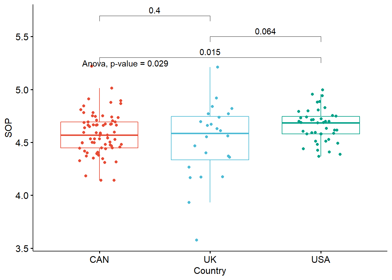
Visulaisation
If you are interested in visualizing results of ANOVA and post-hoc tests on the same plot (directly on the boxplots), here is a piece of code which may be of interest to you:
## set up of elements
x <- which(names(perfectionism) == "Country") # name of independent variable
y <- which(
  names(perfectionism) == "SOP" # name of outcome variable
)
method1 <- "anova" # overall test of main effect = anova
method2 <- "t.test" # test of specific comparisons = t test
my_comparisons <- list(c("CAN", "USA"), c("USA", "UK"), c("UK", "CAN")) # comparisons for post-hoc tests
## building the plot
library(ggpubr)
for (i in y) {
  for (j in x) {
    p <- ggboxplot(perfectionism,
      x = colnames(perfectionism[j]), y = colnames(perfectionism[i]),
      color = colnames(perfectionism[j]),
      legend = "none",
      palette = "npg",
      add = "jitter"
    )
    print(
      p + stat_compare_means(aes(label = paste0(..method.., ", p-value = ", ..p.format..)),
        method = method1, label.y = max(perfectionism[, i], na.rm = TRUE)
      )
      + stat_compare_means(comparisons = my_comparisons, method = method2, label = "p.format")
    )
  }
}
Effect size
We can also calculate effect sizes for the group difference just like we did above.
perfectionism %>%
cohens_d(SOP ~ Country)
## # A tibble: 3 x 7
## .y. group1 group2 effsize n1 n2 magnitude
## * <chr> <chr> <chr> <dbl> <int> <int> <ord>
## 1 SOP CAN UK 0.224 73 24 small
## 2 SOP CAN USA -0.463 73 42 small
## 3 SOP UK USA -0.537 24 42 moderateAccording to Cohen (1988, 1992), the effect size is low if the value of d varies around 0.2, medium if d varies around 0.5, and large if d varies more than 0.8. The UK-USA difference is a large effect and other two comparisons are small effects.
How its written
A one-way between-subjects ANOVA was conducted to compare the effect of country on levels of perfectionism. There was a significant effect of country on perfectionism at the p<.05 level for the three conditions [F(2, 136) = 3.65, p = 0.03]. Post hoc comparisons using the Tukey HSD test indicated that the mean perfectionism score for the US (M = 4.66, SD = 0.16) was significantly larger than the mean perfectionism score for the UK (M = 4.51, SD = 0.35, d=.54). However, the mean perfectionism score for Canada (M = 4.58, SD = 0.20) did not significantly differ from the mean perfectionism scores for the US (d=.46) and the UK (d = .22).
Exercise
Okay, your turn to run some of the tests that we have described here. To do that, let’s once again return to our WVS data and specifically the comparison of perceptions of choice between Australia and Japan that we made last week. Then, we compared the distributions using z-scores. Let’s now go one step further and test the differences in perceptions of choice using a two-parameter linear model or independent t-test.
Before we start, lets just clarify the research question for our two-parameter linear model and null hypothesis we are testing:
Research Question - Do perceptions of choice differ between people from Australia and Japan?
Null Hypothesis - The difference between perceptions of choice in Australia and Japan will be zero.
Task 1 - Loading the dataframe
Load the WVS dataframe. The WVS data is avalaible in the MT9 workshop folder. Load it into the R environment like you have been doing in previous weeks (i.e., click on it, change name to WVS and copy+paste the code below).
WVS <- readRDS("C:/Users/currant/Dropbox/Work/LSE/PB130/MT9/Workshop/WV6_Data_R_v20180912.rds")

WVS$V2A <- as_character(WVS$V2A) # maintain this code for the country variable
Task 2 - Selecting the variables
I looked in the codebook for WVS and the perceptions of choice variable is listed as V55. So lets look for the variable and select it, then head the new dataframe entitled WVSchoice. Lets also select the country code variable, V2A, so we can use this to group the choice scores later. I have left some of the below code blank for you to fill the gap.
WVSchoice <-
  WVS %>%
  select(??, ??) # SELECT THE VARIABLES OF INTEREST HERE
head(WVSchoice)
Task 3 - Filter the variables
Just like other variables in the WVS dataset, we need to edit the dataframe since the choice variable has values we can’t interpret like -5. While we are at it, lets also filter out Australia and Japan as the countries of interest. I have left some of the below code blank for you to fill the gap.
WVSchoice <-
WVSchoice %>%
filter(V55 >= "??" & V2A == c("??", "??")) # Fill in the question marks
WVSchoice
Task 4 - Examine the descriptives
Use the favstats function to inspect the means and SD of the choice scores for Australia and Japan.
favstats(~V55, ??, data=WVSchoice) # Fill in the question markWhat is the mean score for Australia?
What is the mean score for Japan?
Calculate the mean difference
What is the mean difference?
Task 5 - Setting up the linear model
Now lets set our up our linear model to examine the statistical significance of that mean difference. We are using the lm() function to test a two-parameter model because we now have two means to estimate - one for Australia and one for Japan. As I mentioned above, R actually does the dummy coding for us in the lm() function so we don’t need to dummy code the country variable. For noting, R will code Australia as 0 and Japan as 1 (just because thats the order they appear in the data set). Lets just build the model with V2A as the explanatory factor.
choice.model <- lm(V55 ~ 1 + ??, data=WVSchoice) # fill in the variable needed for question mark
summary(choice.model)
What is the mean score for Australia (hint: intercept)?
What is the incremenent needed to find the Japan mean or - put differently - the mean difference?
What is the t-ratio?
What is the p value(remember that e-values mean zero)?
Do we accept or reject the null hypothesis?
Why?
Task 6 - Paritioning variance
We’ve established whether there is a statistically significant mean difference, but how much variance in choice is explained by country? We can answer this question using the supernova() function in R, which breaks down the variance in choice due to the model (ie., country) and error (i.e., variance left over once we’ve subtracted out the model)
supernova(??) # add the choice model you want to examine the varianceWhat is the total variance or sum of squares for perceptions of choice?
How is that sum of squares partitioned between the model?
And the Error?
What is the percentage of variance explained in by the model?
What is the F ratio?
What is the p value?
What do we conclude in relation to our research question?