General Linear Model Diagnostics (LT1)
Preliminaries
library("see")
library("performance")
library("car")
Introduction
The general linear model makes several assumptions about the data at hand. This workshop describes the GLM assumptions for ANOVA and linear regression and provides built-in tools diagnostics in R .
Before performing an analysis using the GLM, you should always check if the model works well for the data at hand: that is to say that key assumptions are met.
For example, the linear regression model makes the assumption that the relationship between the predictors and the outcome variable is linear. This might not be true. The relationship could be polynomial or logarithmic.
Additionally, the data might contain some influential observations, such as outliers (or extreme values), that can affect the result of the regression.
We have covered these topics previously, but it is wise to be aware of them.
In addition to these important topics, as we saw in the lecture, there are other assumptions. These include independence, normality of the residuals and equality of variances.
In this workshop, we’ll look at testing these remaining assumptions in the ANOVA and linear regression models. We’ll finish by describing some built-in diagnostic plots in R.
So lets get started and take a look at diagnostic testing in ANOVA.
ANOVA
Recap: How one-way ANOVA works
ANOVA is a three or more parameter linear model. It tests for differences in one continuous dependent variable on one categorical independent variable with three or more levels.
ANOVA Assumptions
WHat I didn’t tell you last year was that there are a few important assumptions of ANOVA that should be checked before you run the test. I didn’t tell you about these because my core objective was to have you learn the mechanics of the analysis - what is going on under the bonnet.
If on top of all that I tried to teach the diagnostics too, I would have lost you. Just like I was lost when my stats professor taught the analysis and the diagnostics at the same time. The most important thing is to understand the statistics. Once you have done that, we can add on these auxiliary topics.
That is what we are doing today… So what are the assumptions of ANOVA? As we saw in the lecture, there are three main ones:
1. The observations are obtained independently and randomly from the population defined by the factor levels.
What does this mean? Well it means that the data, collected from a representative and randomly selected portion of the total population, should be independent.
The assumption of independence is most often verified based on the design of the experiment and on the good control of experimental conditions rather than via a formal test. If you are still unsure about independence based on the experiment design, ask yourself if one observation is related to another (if one observation has an impact on another) within each group or between the groups themselves. If not, it is most likely that you have independent samples.
If observations between samples (forming the different groups to be compared) are dependent (for example, if three measurements have been collected on the same individuals as it is the case in within-person designs), the repeated measures ANOVA should be preferred in order to take into account the dependency between the samples.
This more of a design issue, and we will talk more about this assumption as we move to multi-level modeling and accounting for independence of observations. But it is important to be aware of it.
2. The data of each factor level are normally distributed.
What does this mean? Well, it means the residuals should follow approximately a normal distribution. This assumption is most important when you have a small sample size (because central limit theorem isn’t working in your favor), and when you’re interested in constructing confidence intervals/doing significance testing.
The normality assumption can be tested visually thanks to a histogram and a QQ-plot, and/or formally via a normality test such as the Shapiro-Wilk or Kolmogorov-Smirnov test.
If, the assumption is violated then the Kruskal-Wallis test can be applied:
kruskal.test(variable ~ group, data = dat in R)
This non-parametric test as we spoke briefly about last year, robust to non-normal distributions, has the same goal as the ANOVA — compare 3 or more groups — but it uses sample medians instead of sample means to compare groups.
Finally, there is also the option of bootstrapping to manage violations of this assumption, which is what we have been doing to date and what we will continue to do.
3. Each level of the factor has common or equality of variance.
What does this mean? Well, it means the variances of the different groups should be equal (an assumption called homogeneity of variances, or even sometimes referred as homoscedasticity, as opposed to heteroscedasticity if variances are different across groups). When this assumption is satisfied, your parameter estimates will be optimal. When there are unequal variances of the dependent variable at different levels of the predictor (i.e., when this assumption is violated), you’ll have inconsistency in your standard error and parameter estimates in your model. Subsequently, your confidence intervals and significance tests will be biased.
This assumption can be tested graphically by comparing the dispersion of each group in a boxplot for instance, or more formally via the Levene’s test:
leveneTest(variable ~ group, data= dat in R)
If the hypothesis of equal variances is rejected, another version of the ANOVA can be used, the Welch test:
oneway.test(variable ~ group, var.equal = FALSE)
Note that the Welch test does not require homogeneity of the variances, but the distributions should still follow approximately a normal distribution.
Testing The ANOVA Assumptions
To give an example of how to test for these assumptions prior to your analyses, we are going to use the perfectionism data from last year. If you remember, this data contain average levels of perfectionism from studies in the US, Canada, and the UK. The focal research question is:
RQ: Do levels of perfectionism differ between samples from the US, Canada and the UK
This is a classic One-Way ANOVA with three levels of the independent variable (Country) and one dependent variable (SOP). We tested this data without testing whether the assumptions of normality and equality of variances were met.
First, lets load this data into our R environment. Go to the LT1 folder, and then to the workshop folder, and find the “perfectionism.csv” file. Click on it and then select “import dataset”. In the new window that appears, click “update” and then when the dataframe shows, click import.
library(readr)## Warning: package 'readr' was built under R version 4.0.3perfectionism <- read_csv("C:/Users/CURRANT/Dropbox/Work/LSE/PB230/LT1/Workshop/perfectionism.csv")##
## -- Column specification -------------------------------------------------------------------------------------------------------------------------------------------------------------
## cols(
## Study = col_character(),
## SOP = col_double(),
## Country = col_character(),
## Region = col_character()
## )head(perfectionism)## # A tibble: 6 x 4
## Study SOP Country Region
## <chr> <dbl> <chr> <chr>
## 1 Hewitt & Flett 4.39 CAN NORTH_AMERICA
## 2 Hewitt & Flett 4.53 CAN NORTH_AMERICA
## 3 Hewitt & Flett 4.45 CAN NORTH_AMERICA
## 4 Westra TH 4.64 CAN NORTH_AMERICA
## 5 Flett 4.57 CAN NORTH_AMERICA
## 6 Flett 4.56 CAN NORTH_AMERICATesting the Assumption of Normality of Residuals
Remember that normality of residuals can be tested visually via a histogram and a QQ-plot, or formally via a normality test (Shapiro-Wilk test, for instance).
Before checking the normality assumption, we first need to compute the ANOVA. We then save the results in res_aov:
anova.model <- aov(SOP ~ Country, data = perfectionism)We can now check normality of the residuals visually:
# histogram
hist(anova.model$residuals)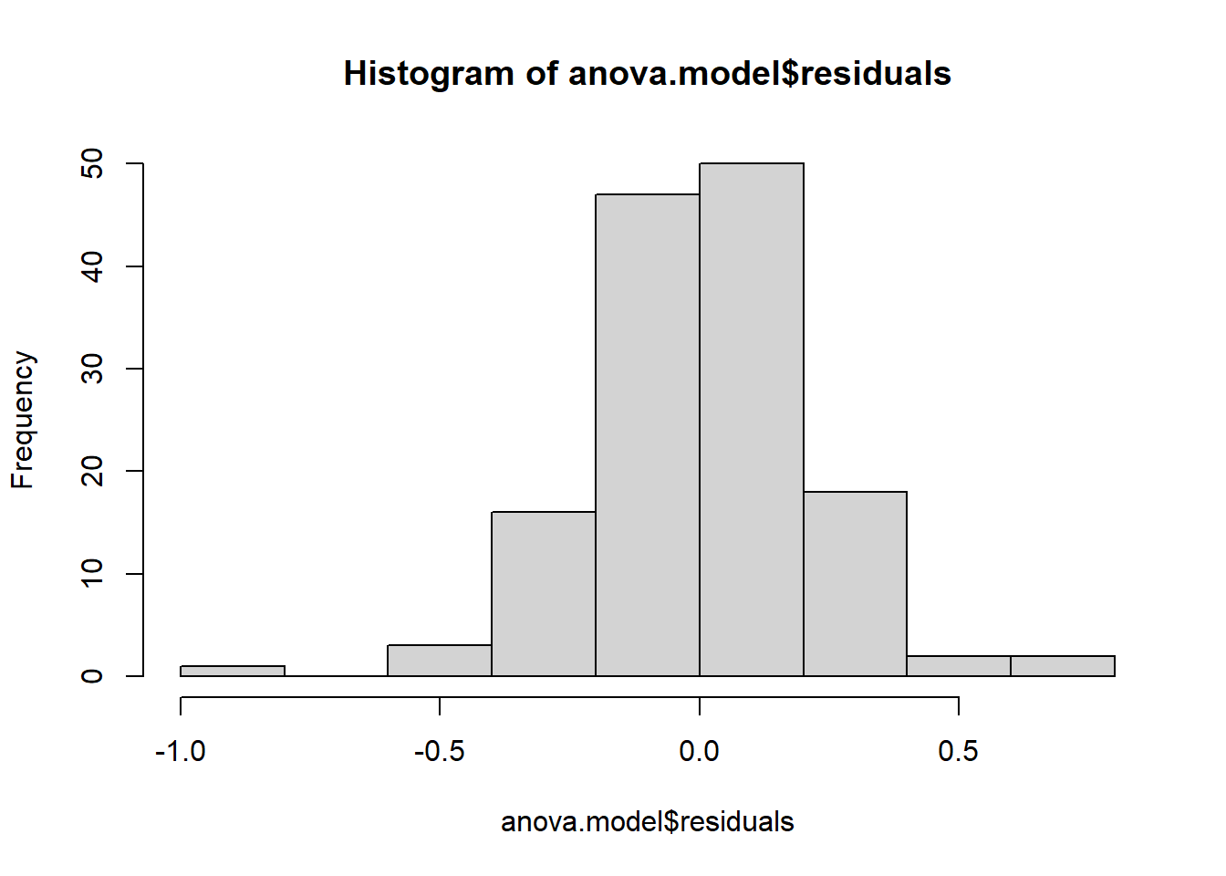
# QQ-plot
library(car)
qqPlot(anova.model$residuals)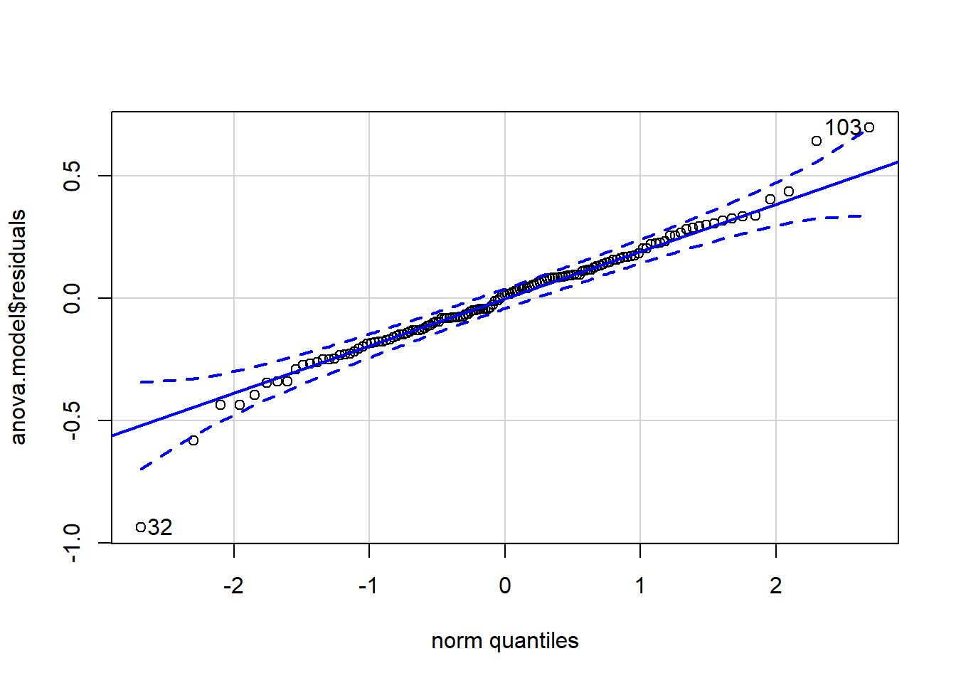
## [1] 32 103From the histogram and QQ-plot above, we can already see that the normality assumption seems to be met. Indeed, the histogram roughly forms a bell curve, indicating that the residuals follow a normal distribution. Furthermore, points in the QQ-plots roughly follow the straight line and most of them are within the confidence bands (there are a couple of outliers that R has flagged: 32 and 103). This also indicates that residuals follow approximately a normal distribution.
Some researchers stop here and assume that normality is met, while others also test the assumption via a formal statistical test. It is your choice to test it (i) only visually, (ii) only via a normality test, or (iii) both visually AND via a normality test. Bear in mind, however, the two following points:
ANOVA is quite robust to small deviations from normality. This means that it is not an issue (from the perspective of the interpretation of the ANOVA results) if a small number of points deviate slightly from the normality.
Normality tests are sometimes quite conservative, meaning that the null hypothesis of normality may be rejected due to a limited deviation from normality. This is especially the case with large samples as power of the test increases with the sample size.
In practice, I tend to prefer the (i) visual approach only, but again, this is a matter of personal choice and also depends on the context of the analysis.
Still for the sake of illustration, we also now test the normality assumption via a normality test. You can use the Shapiro-Wilk test or the Kolmogorov-Smirnov test, among others. Remember that the null and alternative hypothesis are:
H0: data come from a normal distribution
H1: data do not come from a normal distribution
In R, we can test normality of the residuals with the Shapiro-Wilk test thanks to the shapiro.test() function:
shapiro.test(anova.model$residuals)##
## Shapiro-Wilk normality test
##
## data: anova.model$residuals
## W = 0.9716, p-value = 0.005352P-value of the Shapiro-Wilk test on the residuals is smaller than the usual significance level of p = .05. So we reject the hypothesis that residuals follow a normal distribution (p-value = 0.005).
This result contradicts the visual inspection and is evidence that with large samples (i.e., n = 139) the test for normality is highly sensitive to even minor deviations from a normal distribution. This is why I prefer the visual approach to the more formal test when the data “appear” normal.
But this is a good learning opportunity for what to do if the normality assumption is not met. Traditionally researchers have opted to transform data in the hope that residuals would better fit a normal distribution.
But this is non-optimal for a number of reasons including changing the scale of the outcome variable and making model interpretation more difficult.
So we have two options, both involve non-parametric tests (i.e., tests that do not assume a normal distribution.
The first is to bootstrap the estimate and calculate the 95% bootstrap confidence interval. We have been doing this and it is a strategy I recommend.
The second option is to use the non-parametric version of ANOVA: The Kruskal-Wallis test.
kruskal.test(SOP ~ Country, data = perfectionism)##
## Kruskal-Wallis rank sum test
##
## data: SOP by Country
## Kruskal-Wallis chi-squared = 6.5401, df = 2, p-value = 0.038When you carry out a Kruskal-Wallis test you are looking at the ranks of the data and comparing them (rather than the raw units). If the ranks are sufficiently different between samples you may be able to determine that these differences are statistically significant. The F test is replaced by a chi-square value with associated p.
From the output of the Kruskal-Wallis test, we know that there is a significant difference between the countries, but we don’t know which pairs of groups are different.
It’s possible to use the function pairwise.wilcox.test() to calculate non-parametric pairwise comparisons between group levels with corrections for multiple testing.
pairwise.wilcox.test(perfectionism$SOP, perfectionism$Country, p.adjust.method = "BH")## Warning in wilcox.test.default(xi, xj, paired = paired, ...): cannot compute
## exact p-value with ties##
## Pairwise comparisons using Wilcoxon rank sum test with continuity correction
##
## data: perfectionism$SOP and perfectionism$Country
##
## CAN UK
## UK 0.667 -
## USA 0.039 0.138
##
## P value adjustment method: BHAs we saw lat year, the Canada US contrast is significant, (p = .039) but all other contrasts are not different from zero.
Testing Assumption of Equality of Variances
Assuming residuals follow a normal distribution, it is now time to check whether the variances are equal across counties or not. The result will have an impact on whether we use the ANOVA or the Welch test.
This can again be verified visually via a boxplot or more formally via a statistical test.
Visually, we have:
# Boxplot
boxplot(SOP ~ Country, data = perfectionism)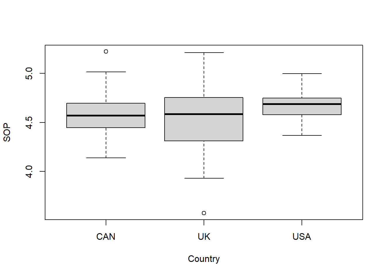
The boxplots show a similar variance for the different countries. This can be seen by the fact that the boxes and the whiskers have a comparable size. However, there are a couple of outliers as shown by the points outside the whiskers and the UK box seems a little fatter (this is likely because the sample size for UK is smaller so therefore more variance).
Like the normality assumption, if you feel that the visual approach is not sufficient, you can formally test for equality of the variances with a Levene’s test. I would suggest there is enough doubt in our box plots to run this test.
The null and alternative hypotheses for the Levene’s test are:
H0: variances are equal H1: at least one variance is different
In R, the Levene’s test can be performed thanks to the leveneTest() function from the {car} package:
# Levene's test
library(car)

leveneTest(SOP ~ Country, data = perfectionism)
## Warning in leveneTest.default(y = y, group = group, ...): group coerced to
## factor.## Levene's Test for Homogeneity of Variance (center = median)
## Df F value Pr(>F)
## group 2 7.8492 0.0005942 ***
## 136
## ---
## Signif. codes: 0 '***' 0.001 '**' 0.01 '*' 0.05 '.' 0.1 ' ' 1The p-value being smaller than the significance level of 0.05, we reject the null hypothesis, so we must reject the hypothesis that variances are equal between groups (p-value = 0.001). It seems the group variances do differ significantly.
An alternative procedure to one-way ANOVA, called the Welch one-way test, does not require the homogeneity of variances assumption to be met. Therefore, if the Levene’s test in significant (i.e., p > .05), researchers should use Welch.
We can implement the Welch’s test using the function oneway.test():
oneway.test(SOP ~ Country, data = perfectionism)##
## One-way analysis of means (not assuming equal variances)
##
## data: SOP and Country
## F = 3.9739, num df = 2.000, denom df = 53.346, p-value = 0.02462The results are similar to what we saw above - the ANOVA is significant (i.e., p < .05). There is a difference.
To examine pairwise t-tests of this model with no assumption of equal variances, we must request the corrected t-tests (for multiple comparisons). But this time we are also going to stipulate that the SDs are not pooled (because the assumption of equal variance has been violated).
Lets do that now:
pairwise.t.test(perfectionism$SOP, perfectionism$Country, p.adjust.method = "BH", pool.sd = FALSE)##
## Pairwise comparisons using t tests with non-pooled SD
##
## data: perfectionism$SOP and perfectionism$Country
##
## CAN UK
## UK 0.404 -
## USA 0.046 0.095
##
## P value adjustment method: BHAs before, this output reveals a similar story. the Canada US contrast is significant, (p = .046) but all other contrasts are not different from zero.
And that’s it! That’s how we diagnose assumptions of ANOVA.
Linear Regression
Recap: How Linear Regression Works
Regression is a infinite parameter linear model. It tests for relationships in one continuous dependent variable on several continuous independent variables.
Linear Regression Assumptions
Because ANOVA and regression ARE THE SAME ANALYSIS, the diagnostic testing follows a similar roadmap.
Let’s review what our linear regression assumptions are conceptually, and then we’ll turn to diagnosing these assumptions in the next section.
1. Linearity. Linear regression is based on the assumption that your model is linear (shocking, I know). Violation of this assumption is very serious: it means that your linear model probably does a bad job at predicting your actual (non-linear) data. Perhaps the relationship between your predictor(s) and criterion is actually curvilinear or cubic.
If that is the case, a linear model does a bad job at modeling that relationship, and it is inappropriate to use such a model. There’s no point in worrying about significance tests or confidence intervals if a linear model doesn’t reflect your non-linear data.
We talked about polynomials last year, so you should know what this means. We formally test linearity at the outset of linear regression analysis.
2. Normally distributed stuff & things. The assumption of normality in regression manifests in two ways:
For significance tests of models to be accurate, the sampling distribution of the thing you’re testing must be normal. Think back the indirect effect. Remember I showed you how the sampling distribution of the indirect effect is positively skewed? This is why we bootstrapped it. Bootstrapping is vital to overcome this assumption - thats why we use it all the time.
To get the best estimates of parameters (i.e., betas in a regression equation), the residuals in the population must be normally distributed. This is exactly the same assumption as we have just tested using ANOVA when we examined the distribution of the residuals.
3. Each level of the continuous predictor has common or equality of variance Equality of variance occurs when the spread of scores for your dependent variable is the same at each level of the predictor. Just as we have just looked at for ANOVA.
4. Independence. Just like ANOVA, independence is similarly important for regression. It means that the errors in your model are not related to each other (i.e., no clustering or repeated measures). Computation of standard error relies on the assumption of independence, so if you don’t have standard error, say goodbye to confidence intervals and significance tests. As I mentioned above, we will look more into this as we move to multi-level modeling. It is a design issue and cannot be tested using stats.
4. No influential outliers. This isn’t technically an assumption of linear regression, but it’s best practice to avoid influential outliers. Why is it problematic to have outliers in your data? Outliers can bias parameter estimates (e.g., mean), and they also affect your sums of squares. Sums of squares are used to estimate the standard error, so if your sums of squares are biased, your standard error likely is too.
It’s really bad to have a biased standard error because it is used to calculate confidence intervals around our parameter estimate. In other words, outliers could lead to biased confidence intervals. Not good and another reason we bootstrap! We need to rid ourselves of those pesky outliers. We looked at this topic in depth last semester when we cleaned the dataset and inspected for missing data and outliers. So make sure you always do a good job of cleaning and screening before you begin analyses!
Testing The Linear Regression Assumptions
To practice diagnosing a linear regression model with continuous variables (simple regression), we are going to use the happiness and GDP variables in the WHR dataframe. Remember this data from last year? Our theory was that as the wealth of a country increases, so self-report happiness also increases. In other words, we are expecting a positive relationship between wealth as measured by GDP and happiness as measured by the Cantril life ladder.
Before we delve into this topic, lets just clarify the research question we are testing:
RQ: Is there a linear relationship between GDP and happiness?
First, lets load this data into our R environment. Go to the LT2 folder, and then to the workshop folder, and find the “WHR.csv” file. Click on it and then select “import dataset”. In the new window that appears, click “update” and then when the dataframe shows, click import.
WHR <- read_csv("C:/Users/CURRANT/Dropbox/Work/LSE/PB230/LT1/Workshop/WHR.csv")##
## -- Column specification -------------------------------------------------------------------------------------------------------------------------------------------------------------
## cols(
## Country = col_character(),
## Year = col_double(),
## Happiness = col_double(),
## GDP = col_double(),
## GINI = col_double()
## )head(WHR)## # A tibble: 6 x 5
## Country Year Happiness GDP GINI
## <chr> <dbl> <dbl> <dbl> <dbl>
## 1 Afghanistan 2008 3.72 7.17 NA
## 2 Afghanistan 2009 4.40 7.33 NA
## 3 Afghanistan 2010 4.76 7.39 NA
## 4 Afghanistan 2011 3.83 7.42 NA
## 5 Afghanistan 2012 3.78 7.52 NA
## 6 Afghanistan 2013 3.57 7.52 NABefore we begin, lets just filter the GDP variable to get rid of the cases with missing values.
library(tidyverse)## Warning: package 'tidyverse' was built under R version 4.0.3## -- Attaching packages -------------------------------------------------------------------------------------------------------------------------------------------- tidyverse 1.3.0 --## v ggplot2 3.3.3 v dplyr 1.0.2
## v tibble 3.0.3 v stringr 1.4.0
## v tidyr 1.1.2 v forcats 0.5.0
## v purrr 0.3.4## Warning: package 'ggplot2' was built under R version 4.0.3## -- Conflicts ----------------------------------------------------------------------------------------------------------------------------------------------- tidyverse_conflicts() --
## x dplyr::filter() masks stats::filter()
## x dplyr::lag() masks stats::lag()
## x dplyr::recode() masks car::recode()
## x purrr::some() masks car::some()WHR <- # into existing dataframe
WHR %>% # from existing daraframe
filter(GDP >= "1") # Filter GDP at a value of 1 and above (i.e., rid the dataframe of any non-numeric cases)
head(WHR)## # A tibble: 6 x 5
## Country Year Happiness GDP GINI
## <chr> <dbl> <dbl> <dbl> <dbl>
## 1 Afghanistan 2008 3.72 7.17 NA
## 2 Afghanistan 2009 4.40 7.33 NA
## 3 Afghanistan 2010 4.76 7.39 NA
## 4 Afghanistan 2011 3.83 7.42 NA
## 5 Afghanistan 2012 3.78 7.52 NA
## 6 Afghanistan 2013 3.57 7.52 NAThen lets run the linear model:
lm.model<-lm(Happiness~GDP, data=WHR)
summary(lm.model)
##
## Call:
## lm(formula = Happiness ~ GDP, data = WHR)
##
## Residuals:
## Min 1Q Median 3Q Max
## -2.31546 -0.48824 -0.03528 0.54885 2.01733
##
## Coefficients:
## Estimate Std. Error t value Pr(>|t|)
## (Intercept) -1.35609 0.13476 -10.06 <2e-16 ***
## GDP 0.73685 0.01449 50.84 <2e-16 ***
## ---
## Signif. codes: 0 '***' 0.001 '**' 0.01 '*' 0.05 '.' 0.1 ' ' 1
##
## Residual standard error: 0.7034 on 1674 degrees of freedom
## Multiple R-squared: 0.6069, Adjusted R-squared: 0.6067
## F-statistic: 2585 on 1 and 1674 DF, p-value: < 2.2e-16As we saw last year, these variables share a significant positive relationship (b = .74, p < .001).
Testing for linearity and equality of variances
To test for linearity and equality of variances we plot the fitted values (predicted values) against the residuals.
The plot of residuals versus predicted values is useful for checking the assumption of linearity and equality of variances. If the model does NOT meet the linear model assumption, we would see our residuals take on a defined shape or a distinctive pattern. For example, if your plot looks like a parabola, that’s bad.
Your scatterplot of residuals should look like the night sky–no distinctive patterns. The red line through your scatterplot should also be straight and horizontal, not overly curved, if the linearity assumption is satisfied.
To assess if the equality of variances assumption is met we look to make sure that the residuals are equally spread around the y = 0 line.
plot(lm.model,which=1)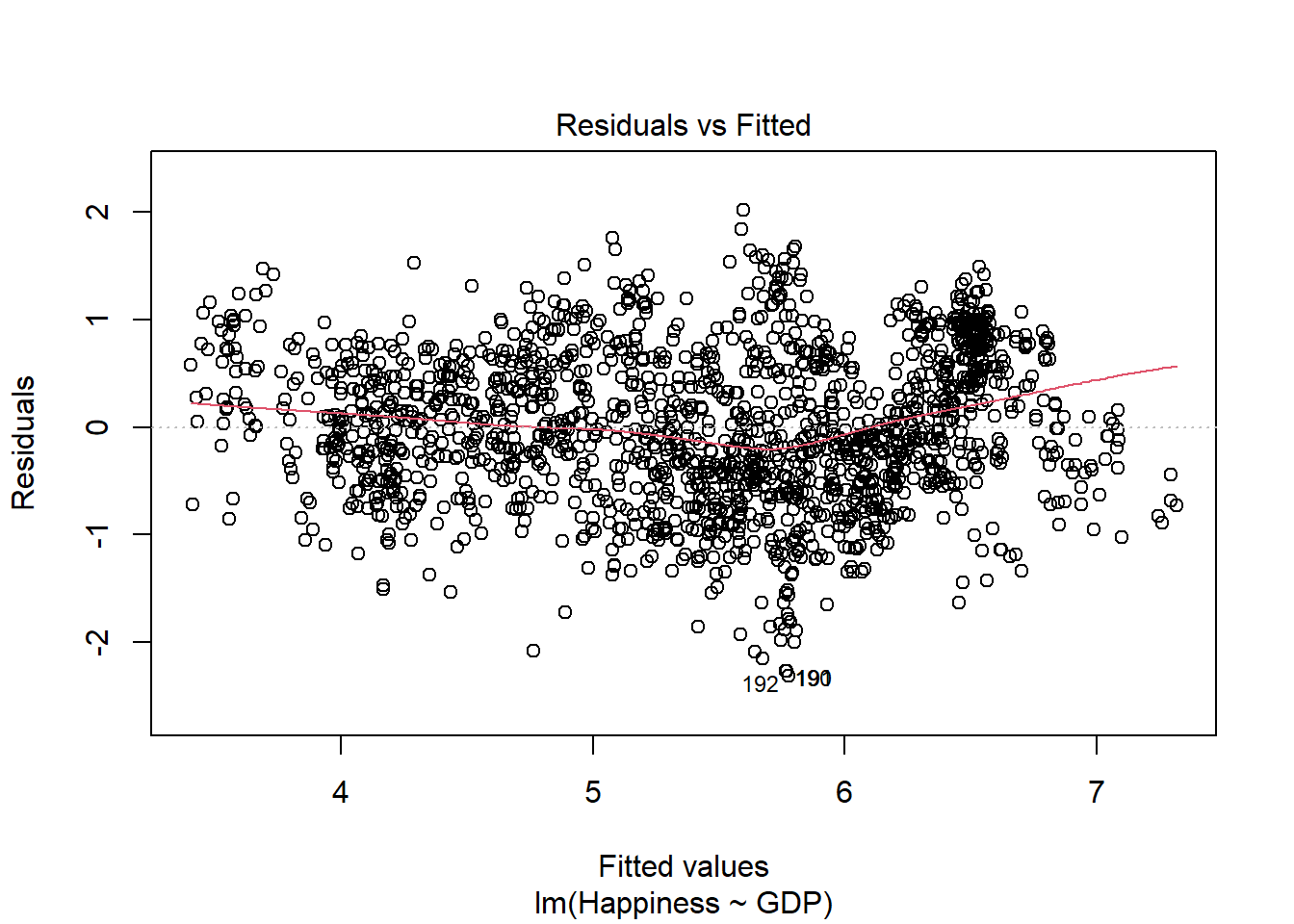
How did we do? R automatically flagged 2 data points that have large residuals (observations 192 and 190). Besides that, our residuals appear to be pretty linear, as is evidenced by the almost straight red line plotted through our residuals (if they were quadratic, for example, that line would resemble the shape of a parabola). It also looks like our data have equal variance across the range of the predictor, given that they appear evenly spread around the y = 0 line. Hooray!
Testing for Normality of Residuals
Just like ANOVA, the normality assumption is evaluated based on the residuals and can be evaluated using a histogram and QQ-plot. The QQ-Plot, to remind you, plots the standardized residuals against a perfect normal distribution of theoretical quantiles. If there is a perfect, or near perfect, linear relation then the residuals are indeed normally distributed.
# histogram
hist(lm.model$residuals)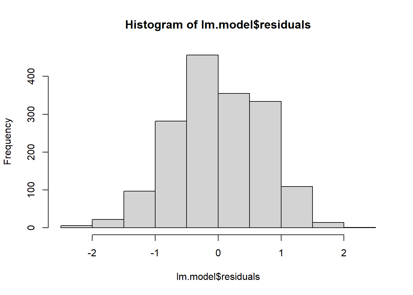
# QQ-plot
library(car)
qqPlot(lm.model$residuals) 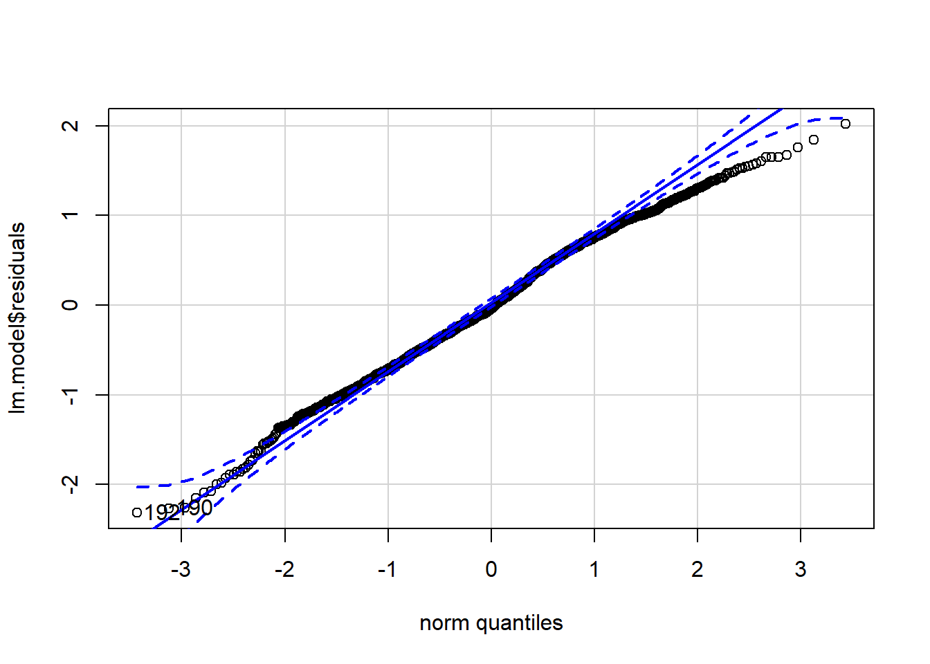
## [1] 192 190How did we do? R automatically flagged those same 2 data points that have large residuals (observations 192 and 190). However, aside from those 2 data points, observations lie well along the 45-degree line in the QQ-plot, and the histogram has a nice bell shape, so we may assume that normality holds here.
We could test this more formally, as we did for ANOVA. But regression is robust to small deviations in normality and, besides, our sample so large it will invariably turn a significant result. No need here. The residuals look pretty symmetrical.
Awesome! Job done, we are good to carry on with the analysis.
Global Tests of Linear Model Assumptions
Finally, I found a really cool package this week that tests model assumptions simultaneously. It is called performance and it is kickass.
We can check out (almost) everything using just one package using the check_model() function. Lets do that now for out ANOVA and regression models
library(performance)
check_model(anova.model)
## `geom_smooth()` using formula 'y ~ x'
## `geom_smooth()` using formula 'y ~ x'## Warning in simpleLoess(y, x, w, span, degree = degree, parametric =
## parametric, : pseudoinverse used at 4.5126## Warning in simpleLoess(y, x, w, span, degree = degree, parametric =
## parametric, : neighborhood radius 0.14653## Warning in simpleLoess(y, x, w, span, degree = degree, parametric =
## parametric, : reciprocal condition number 4.1964e-015## Warning in simpleLoess(y, x, w, span, degree = degree, parametric =
## parametric, : There are other near singularities as well. 0.0068695## `geom_smooth()` using formula 'y ~ x'## Warning in simpleLoess(y, x, w, span, degree = degree, parametric =
## parametric, : pseudoinverse used at 4.5126## Warning in simpleLoess(y, x, w, span, degree = degree, parametric =
## parametric, : neighborhood radius 0.14653## Warning in simpleLoess(y, x, w, span, degree = degree, parametric =
## parametric, : reciprocal condition number 4.1964e-015## Warning in simpleLoess(y, x, w, span, degree = degree, parametric =
## parametric, : There are other near singularities as well. 0.0068695## `stat_bin()` using `bins = 30`. Pick better value with `binwidth`.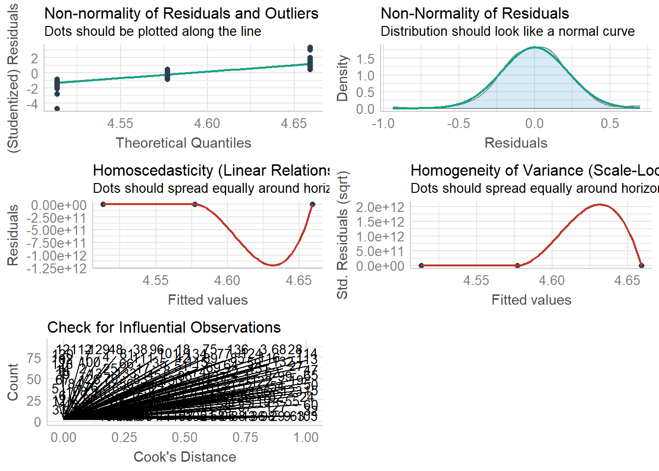
check_model(lm.model)## `geom_smooth()` using formula 'y ~ x'
## `geom_smooth()` using formula 'y ~ x'
## `geom_smooth()` using formula 'y ~ x'
## `stat_bin()` using `bins = 30`. Pick better value with `binwidth`.## Warning: Removed 1676 rows containing missing values (geom_text_repel).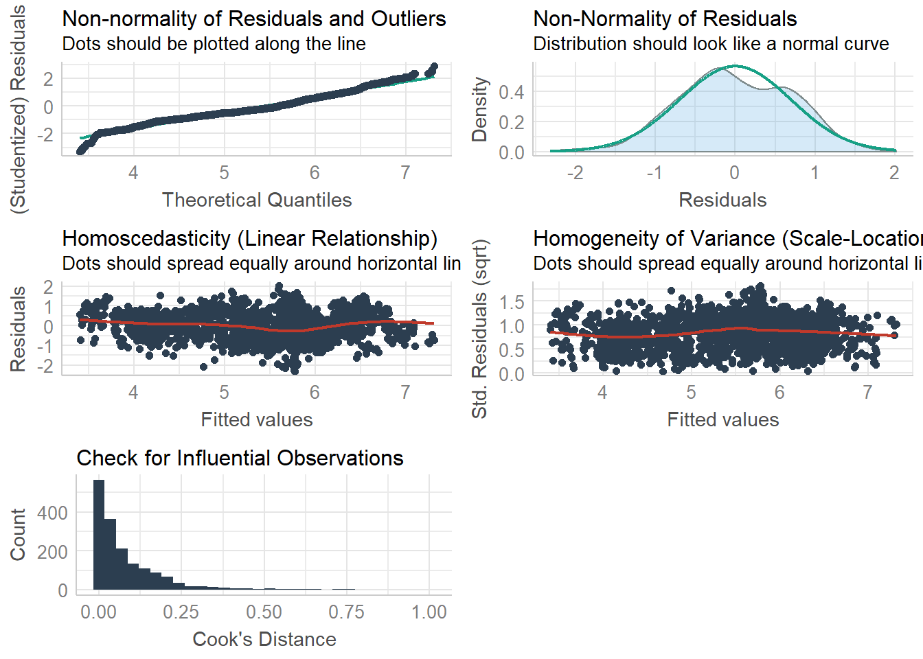
Just as the other plots suggested, all of our assumptions seem to be acceptable for the linear regression model. But there are some issue of homogeneity identified for the ANOVA (which we addressed).
Activity
Okay, lets do some diagnosis on some ANOVA data to give you a chance to practice.
The data are taken from last years secondary data assignment. If you remember, I gave you some data from an online retailer interested in improving their workers’ productivity at work with music. To test whether music had an impact on productivity, a researcher recruited a sample of 150 and randomly split them into three groups:
a “control group” that did not listen to music (no_music)
a “treatment group” who listened to music, but had no choice of what they listened to (music_no_choice)
a second treatment group who listened to music and had a choice of what they listened to (music_choice)
After a month of intervention, productivity was measured.
The research question was:
RQ: Is there a statistically significant difference in productivity between the three conditions?
You task is to diagnose this data for normality of residuals and equality of variance.
First lets load in the data:
music_data <- read_csv("C:/Users/CURRANT/Dropbox/Work/LSE/PB230/LT1/Workshop/music_data.csv")##
## -- Column specification -------------------------------------------------------------------------------------------------------------------------------------------------------------
## cols(
## ID = col_double(),
## condition = col_character(),
## productivity = col_double()
## )head(perfectionism)## # A tibble: 6 x 4
## Study SOP Country Region
## <chr> <dbl> <chr> <chr>
## 1 Hewitt & Flett 4.39 CAN NORTH_AMERICA
## 2 Hewitt & Flett 4.53 CAN NORTH_AMERICA
## 3 Hewitt & Flett 4.45 CAN NORTH_AMERICA
## 4 Westra TH 4.64 CAN NORTH_AMERICA
## 5 Flett 4.57 CAN NORTH_AMERICA
## 6 Flett 4.56 CAN NORTH_AMERICATask 1: Setting up the Model
In the chunk below, write the code to create the build the ANOVA model using aov. Save the model as “music.model”
music.model <- aov(productivity ~ condition, data = music_data)Task 2: Plot the normality of residuals
Use the below chunk to write the code to plot a histogram and QQ-plot for the residuals.
# histogram
hist(music.model$residuals)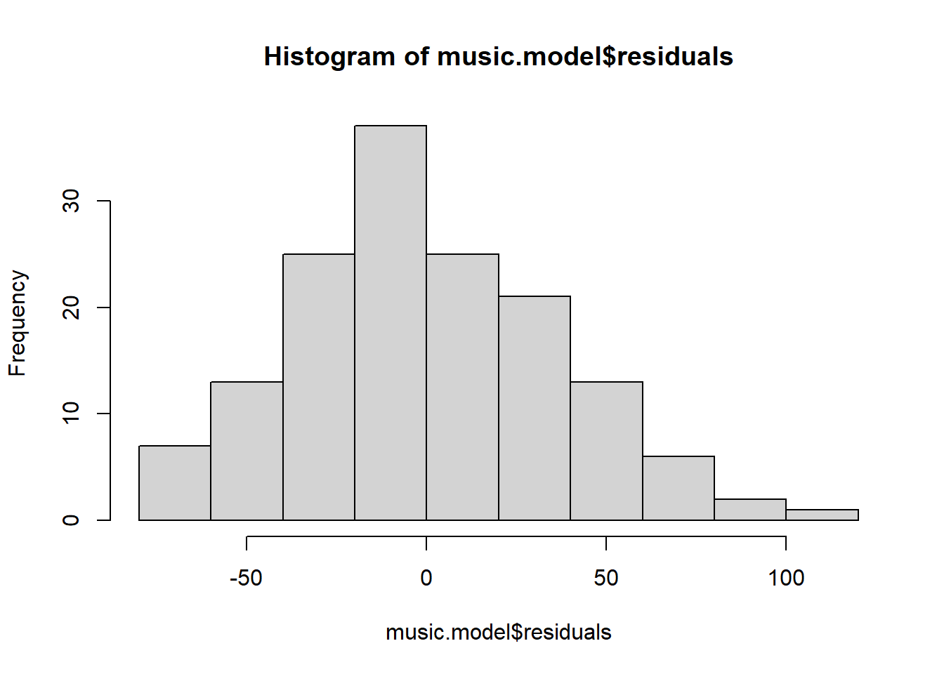
# QQ-plot
qqPlot(music.model$residuals) 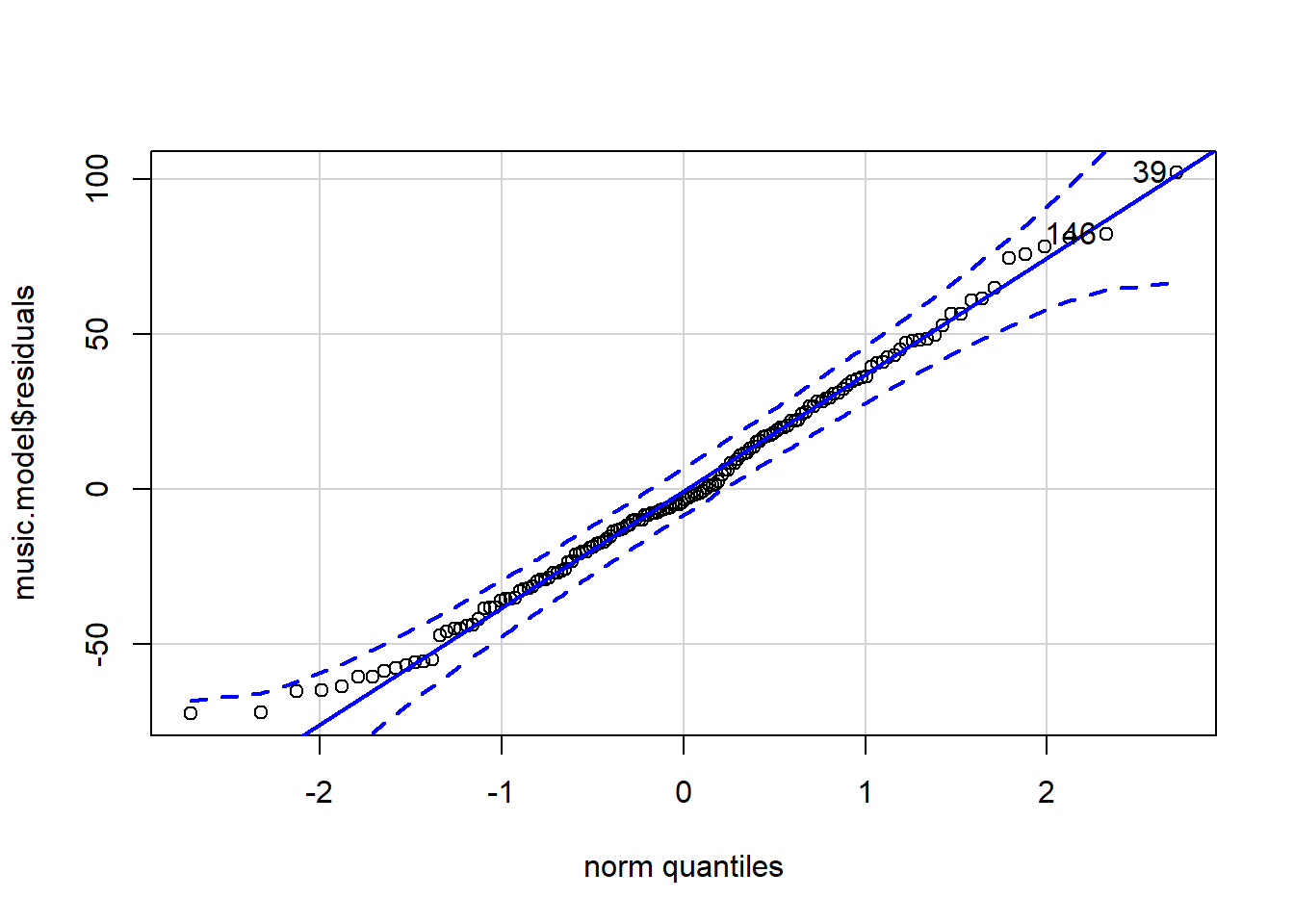
## [1] 39 146What can we say about the normality of the residuals from a visual inspection?
Task 3: Test the normality of residuals
Use the below chunk to write the code for the Shapiro-Wilk test for normality
shapiro.test(music.model$residuals)##
## Shapiro-Wilk normality test
##
## data: music.model$residuals
## W = 0.98934, p-value = 0.3128What can we say about the normality of the residuals from this analysis?
Task 4: Plot the equaltiy of variance
In the chunk below write the code to plot the distributions of the conditions in this experiment using box-plots.
boxplot(productivity ~ condition, data = music_data)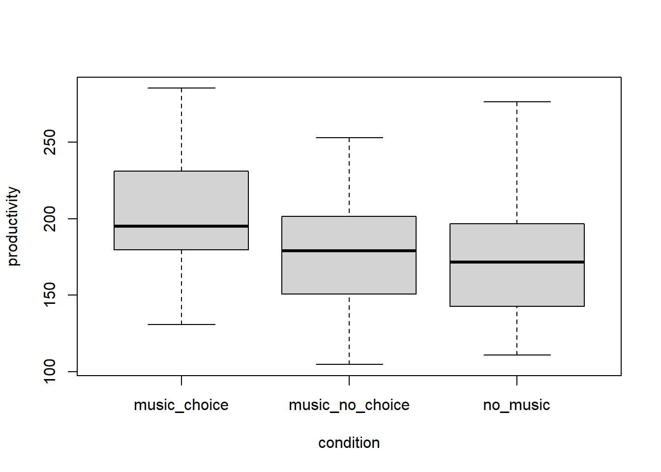
What can we say about the equality of variances from a visual inspection?
Task 5: Test the homogenity of variances
Use the below chunk to write the code for the Levene’s test of equality of variances.
leveneTest(productivity ~ condition, data = music_data)## Warning in leveneTest.default(y = y, group = group, ...): group coerced to
## factor.## Levene's Test for Homogeneity of Variance (center = median)
## Df F value Pr(>F)
## group 2 0.6211 0.5388
## 147What can we say about the equality of variances from this analysis?