Exploratory and Confirmatory Factor Anaysis (LT3)
Preliminaries
library(corpcor)
library(GPArotation)
library(psych)
library(tidyverse)
library(lavaan)
library(semPlot)
The Scourge of Measurement Error
Regression and related techniques (e.g. ANOVA) under the umbrella of the general linear model require us to assume that our measured variables are good indices of these underlying constructs, and that they are measured without any error.
When outcomes are straightforward observed variables like height or weight, and where predictors are experimentally manipulated, then these assumptions are reasonable. However in many applied fields these are not reasonable assumptions to make.
For example, to assume that depression or working memory are indexed in a straightforward way by responses to a depression questionnaire or performance on a laboratory task is naive. Self-reported instruments force participants to approximate and recall. Participants may read the questions wrong. Researchers may code responses incorrectly. In fact, there are a multitude of reasons why a persons score on a measured variable may not reflect the true score.
Perfect measurement is rare to impossible – especially in psychology.
Measurement Theory
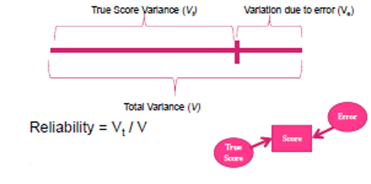
Classic measurement theory says there are two portions of variance in measured variables:
the ‘true score variance’, quantifying the actual construct of interest, and
the ‘error variance’, measuring the variation due to imperfect measurement.
Error variance places an upper limit on correlation because it is assumed to be irrelevant to the outcome. As such, measurement error attenuates relationships and biases findings.
Measurement error can be quantified by the proportion of the ‘true score variance’ to the ‘total variance’, where the total variance is 1.
The higher the reliability, the lower the error. We saw this last yrear when we looked at the reliability of our psychological measures
Reliability
There is, though, a better way to take into account measurement error than reliability. In classic measurement theory, reliability is considered as a subset of validity.
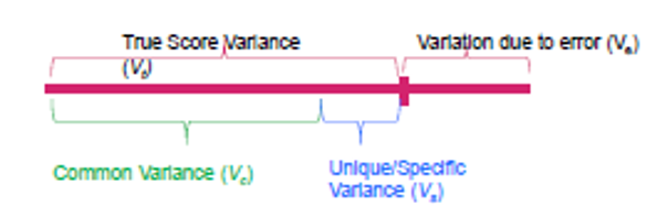
When measurements have multiple indicators, each indicator will contain its own specific variance, but it will also contain variance common to the other indicators.
It is this common variance that speaks to the ‘true’ construct of interest.
Validity
If we strip away the unique variance of a set of items, we are left with their common variance, which is necessarily measured without error.
So by taking the common variance of a set of items we will be much closer to construct we are interested in (i.e., we have rid it of invalidity and unreliability).
This common variance hence reflects the ‘true’ construct score. And becasue it is the true construct score, it is measured without error!
How, then, to capture the common variance of items? With latent variables!
We have noted that construct measurement has error variance, unique variance, and common variance.
We can represent these sources of variance in a latent variable as such:
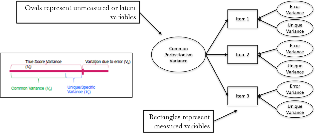
A Latent Variable
These are sometimes called factors or latent factors. Typically you will see them referred to as latent variables, though. The common variance of the items is captured in the latent (oval) variable. What is left, the residual of each item, captures the error variance.
Two statistical methods are avalaible to us in the analysis of measurement using latent variables.
Exploratory Factor Analysis if the factor structure of the items is unknown
Confirmatory Factor Analysis if the factor structure of the items is known
Let’s begin with Exploratory Factor Analysis
Exploratory Factor Analysis (EFA)
What is EFA?
In psychology, we often try to measure things that cannot directly be measured. For example, management researchers might be interested in measuring ‘burnout’, which is when someone who has been working very hard on a project for a prolonged period of time suddenly finds themselves devoid of motivation and inspiration.
You cannot measure burnout directly: it has many facets. However, you can measure different aspects of burnout. You could get some idea of motivation, stress levels, and so on.
Having done this, it would be helpful to know whether these differences really do reflect a single variable. Put another way, are these different variables driven by the same underlying variable?
Factor analysis (and Principal Components Analysis) is a technique for identifying groups or clusters of variables for a pool of items.
Clusters of Items Refecting the Different Factors of Burnout
EFA is an exploratory technique because it does not assume a factor structure for the items. It starts with the assumption of hidden latent variables which cannot be observed directly but are reflected in the answers the items in our questionnaire.
In this way, EFA finds the most optimal factor structure from the underlying items.
What is a Factor?
If we take several items on a questionnaire, the correlation between each pair of items can be arranged in what’s known as an R-matrix. An R-matrix is just a correlation matrix: a table of correlation coefficients between variables.
The diagonal elements of an R-matrix are all 1 because each variable will correlate perfectly with itself. The off-diagonal elements are the correlation coefficients between pairs of items.
The existence of clusters of large correlation coefficients between subsets of variables suggests that those variables could be measuring aspects of the same underlying dimension. These underlying dimensions are known as factors (or latent variables, same thing).
By reducing a data set from a items into a smaller set of factors, factor analysis achieves parsimony by explaining the maximum amount of common variance in a correlation matrix using the smallest number of explanatory constructs.
In other words, factors are a small set of clusters of interrelated items that can explain most of the common variance.
What is a Factor Loading?
If we visualize factors as classification axes, then each variable can be plotted along with each classification axis. For example, two factors (e.g., “Sociability” and “Consideration”) can be plotted as a 2D graph, while six variables (e.g., “Selfish”) can be put at corresponding positions on the graph, as shown below. Such factor plot can be drawn after two factors have been extracted via techniques described in later section that best summarize the items into two clusters.
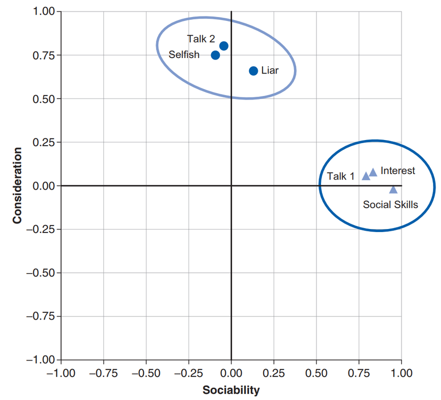
EFA
A factor loading means the coordinate of a item along a classification axis for extracted factors. The factor loading can be thought of as the Pearson correlation between a factor and a variable. You know what that is!
What is communality?
The total variance for a particular item, as we have seen, will have two components: some of it will be shared with other variables or measures (common variance) and some of it will be specific to that measure (unique variance).
We tend to use the term unique variance to refer to variance that can be reliably attributed to only one item. However, again as we know, there is also variance that is specific to one item but not reliably so. This variance is called error variance and is what is left after common variance and unique variance are subtracted out.
The proportion of common variance present in an item is known as the communality. As such, an item that has no unique or error variance would have a communality of 1, an item that shares none of its variance with any other variable would have a communality of 0.
In factor analysis we are interested in finding common underlying dimensions within the data and so we are primarily interested only in the common variance. Therefore, when we run a factor analysis it is fundamental that we know how much of the variance present in our data is common variance.
How to Calculate Communality?
There are various methods of estimating communalities, but the most widely used is to use the squared multiple correlation (SMC) of each variable with all others. So, for the popularity data, imagine you ran a multiple regression using one measure (Selfish) as the outcome and the other five measures as predictors: the resulting multiple R2 would be used as an estimate of the communality for the variable Selfish. This second approach is used in factor analysis.
Factor analysis vs. Principal Components Analysis (PCA)
Strictly speaking, what we are working with in this unit is PCS not factor analysis. Factor analysis derives a mathematical model from which factors are estimated, whereas PCA merely decomposes the original data into a set of optimally weighted latent variables (much like multiple regression!)
Because PCA is a perfectly good procedure and conceptually less complex than factor analysis, we are going to work with it here.
PCA combines common and specific variance into explained variance. The total item variance is used in the positive diagonal of the observed correlation matrix before factor extraction. It finds components that maximize the amount of the total variance that is explained.
PCA aims to identify a new smaller set of latent variables, called principal components, that explain the total variance. PCA assumes that this total variance reflects the sum of explained and error variance. Each principle component is a linear function of the original variables.
For example, lets say we have 12 items for our new questionnaire, each are standardized with a sum of squares of 1. In total, our data set contains 12 items with 12 sum of squares.
If we pool all the items into one factor, we explain half of the variance in the dataset (i.e., explained variance = 6 sum of squares, error variance = 6 sum of squares). If we were to split the items across two factors, we explain a further 4 sum of squares (i.e., explained variance = 10 sum of squares, error variance 2 sum of squares). If we further split the items across three factors we explain all the variance in the data set (i.e., explained variance = 12 sum of squares, error variance 0 sum of squares. The three factors can replace the 12 items without losing any information. This is goal of factor analysis
However, it is rarely this simple. There will always be some error variance unless the number of factors extracted equals the number of items. So the question is: when to stop? When do we have a factor structure that most parsimoniously describes the interrelationships between the items?
There are a variety of approaches to determine the number of factors to extract. These include:
The percentage of variance explained, e.g. stop at 75%
A priori criterion, i.e., a decision is made to identify a particular number of vectors.
Kaiser’s (1960) stopping rule. Extract only factors with an eigenvalue of 1 or more. An eignenvalue is variance explained, bit like standardised sum of squares.
Inspect a Scree Plot for the critical inflection point (Cattell, 1958).
We are going to use methods 3 and 4 because they are the more universally accepted.
Factor Rotation
Once factors have been extracted, it is possible to calculate the factor loading.
Generally, you will find that most variables have high loadings on the most important factor and small loadings on all other factors. This characteristic makes interpretation difficult, and so a technique called factor rotation is used to discriminate between factors. If a factor is a classification axis along which variables can be plotted, then factor rotation effectively rotates these factor axes such that variables are loaded maximally on only one factor.
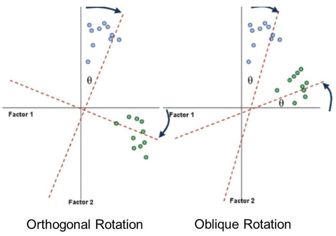
Factor Rotation
There are two types of rotation that can be done. The first is orthogonal rotation while the other is oblique rotation. The difference with oblique rotation is that the factors are allowed to correlate. We will use orthogonal rotation here, sometimes called varimax rotation.
Example: Anxiety Questionnaire
The main usage of factor analysis is the psychological and behavioral scientists is to develop questionnaires. If we want to measure something, we need to ensure that the questions asked relate to the construct that we intend to measure.
Below is the screen shot of a questionnaire of statistics anxiety (copied from the Andy Field’s book):
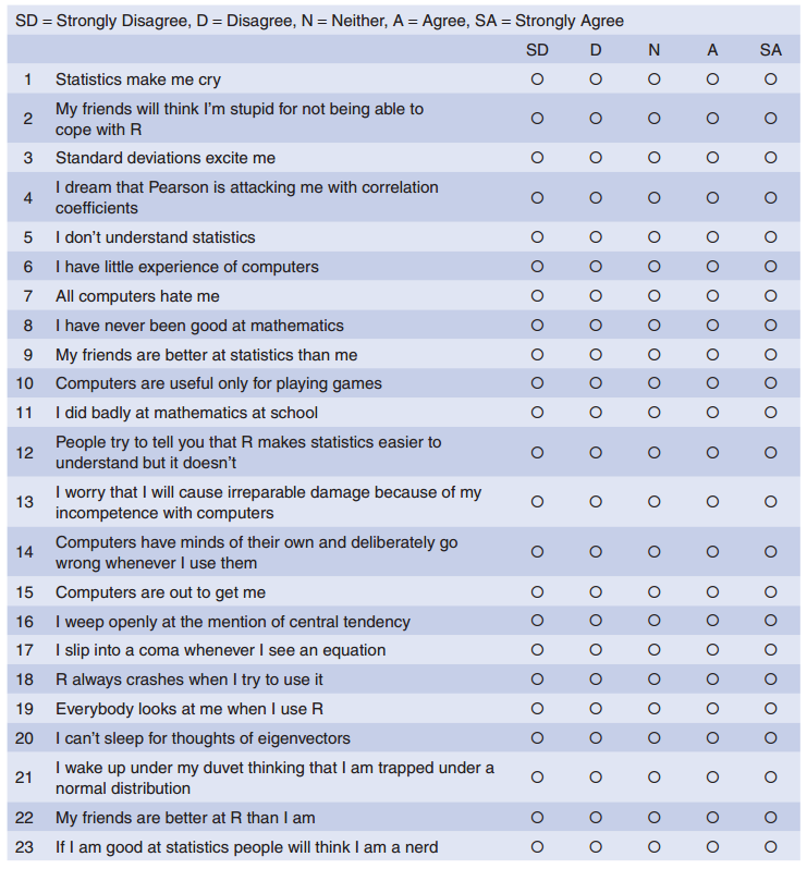
Anxiety Questionnaire
The questionnaire was designed to predict how anxious a given individual would be about learning how to use R. What’s more, they wanted to know whether anxiety about R could be broken down into specific forms of anxiety. In other words, what latent variables contribute to anxiety about R?
With a little help from a few lecturer friends the researcher collected 2571 completed questionnaires (at this point it should become apparent that this example is fictitious). We are going to work with this data today.
Lets load the data into R
library(readr)
anxiety <- read_csv("C:/Users/CURRANT/Dropbox/Work/LSE/PB230/LT3/Workshop/anxiety.csv")
## Warning: Missing column names filled in: 'X1' [1]##
## -- Column specification ---------------------------------------------------------------------
## cols(
## .default = col_double()
## )
## i Use `spec()` for the full column specifications.head(anxiety)## # A tibble: 6 x 24
## X1 Q01 Q02 Q03 Q04 Q05 Q06 Q07 Q08 Q09 Q10 Q11 Q12
## <dbl> <dbl> <dbl> <dbl> <dbl> <dbl> <dbl> <dbl> <dbl> <dbl> <dbl> <dbl> <dbl>
## 1 1 4 5 2 4 4 4 3 5 5 4 5 4
## 2 2 5 5 2 3 4 4 4 4 1 4 4 3
## 3 3 4 3 4 4 2 5 4 4 4 4 3 3
## 4 4 3 5 5 2 3 3 2 4 4 2 4 4
## 5 5 4 5 3 4 4 3 3 4 2 4 4 3
## 6 6 4 5 3 4 2 2 2 4 2 3 4 2
## # ... with 11 more variables: Q13 <dbl>, Q14 <dbl>, Q15 <dbl>, Q16 <dbl>,
## # Q17 <dbl>, Q18 <dbl>, Q19 <dbl>, Q20 <dbl>, Q21 <dbl>, Q22 <dbl>, Q23 <dbl>You will see that the dataset contains responses to 23 items regarding R anxiety. Great we can get started factor analyzing to see whether we can identify the optimal factor structure from the underlying items.
Correlations Between Items
The first thing to do when conducting a factor analysis or PCA is to look at the correlations of the variables. The correlations between variables can be checked using the cor() function to create a correlation matrix of all variables.
There are essentially two potential problems:
1. Correlations are not high enough. We can test this problem by visually scanning the correlation matrix and looking for correlations below about .3. If any variables have lots of correlations below this value then consider excluding them.
2. Correlations are too high. For this problem, if you have reason to believe that the correlation matrix has multicollinearity then you could look through the correlation matrix for variables that correlate very highly (R > .8) and consider eliminating one of the variables (or more) before proceeding.
Lets run-off the correlations now:
anxiety.cor <-
  anxiety %>%
  select(2:24)
cor.matrix <- cor(anxiety.cor)
(round(cor.matrix, 2))
## Q01 Q02 Q03 Q04 Q05 Q06 Q07 Q08 Q09 Q10 Q11 Q12
## Q01 1.00 -0.10 -0.34 0.44 0.40 0.22 0.31 0.33 -0.09 0.21 0.36 0.35
## Q02 -0.10 1.00 0.32 -0.11 -0.12 -0.07 -0.16 -0.05 0.31 -0.08 -0.14 -0.19
## Q03 -0.34 0.32 1.00 -0.38 -0.31 -0.23 -0.38 -0.26 0.30 -0.19 -0.35 -0.41
## Q04 0.44 -0.11 -0.38 1.00 0.40 0.28 0.41 0.35 -0.12 0.22 0.37 0.44
## Q05 0.40 -0.12 -0.31 0.40 1.00 0.26 0.34 0.27 -0.10 0.26 0.30 0.35
## Q06 0.22 -0.07 -0.23 0.28 0.26 1.00 0.51 0.22 -0.11 0.32 0.33 0.31
## Q07 0.31 -0.16 -0.38 0.41 0.34 0.51 1.00 0.30 -0.13 0.28 0.34 0.42
## Q08 0.33 -0.05 -0.26 0.35 0.27 0.22 0.30 1.00 0.02 0.16 0.63 0.25
## Q09 -0.09 0.31 0.30 -0.12 -0.10 -0.11 -0.13 0.02 1.00 -0.13 -0.12 -0.17
## Q10 0.21 -0.08 -0.19 0.22 0.26 0.32 0.28 0.16 -0.13 1.00 0.27 0.25
## Q11 0.36 -0.14 -0.35 0.37 0.30 0.33 0.34 0.63 -0.12 0.27 1.00 0.34
## Q12 0.35 -0.19 -0.41 0.44 0.35 0.31 0.42 0.25 -0.17 0.25 0.34 1.00
## Q13 0.35 -0.14 -0.32 0.34 0.30 0.47 0.44 0.31 -0.17 0.30 0.42 0.49
## Q14 0.34 -0.16 -0.37 0.35 0.32 0.40 0.44 0.28 -0.12 0.25 0.33 0.43
## Q15 0.25 -0.16 -0.31 0.33 0.26 0.36 0.39 0.30 -0.19 0.30 0.36 0.33
## Q16 0.50 -0.17 -0.42 0.42 0.39 0.24 0.39 0.32 -0.19 0.29 0.37 0.41
## Q17 0.37 -0.09 -0.33 0.38 0.31 0.28 0.39 0.59 -0.04 0.22 0.59 0.33
## Q18 0.35 -0.16 -0.38 0.38 0.32 0.51 0.50 0.28 -0.15 0.29 0.37 0.49
## Q19 -0.19 0.20 0.34 -0.19 -0.17 -0.17 -0.27 -0.16 0.25 -0.13 -0.20 -0.27
## Q20 0.21 -0.20 -0.32 0.24 0.20 0.10 0.22 0.18 -0.16 0.08 0.26 0.30
## Q21 0.33 -0.20 -0.42 0.41 0.33 0.27 0.48 0.30 -0.14 0.19 0.35 0.44
## Q22 -0.10 0.23 0.20 -0.10 -0.13 -0.17 -0.17 -0.08 0.26 -0.13 -0.16 -0.17
## Q23 0.00 0.10 0.15 -0.03 -0.04 -0.07 -0.07 -0.05 0.17 -0.06 -0.09 -0.05
## Q13 Q14 Q15 Q16 Q17 Q18 Q19 Q20 Q21 Q22 Q23
## Q01 0.35 0.34 0.25 0.50 0.37 0.35 -0.19 0.21 0.33 -0.10 0.00
## Q02 -0.14 -0.16 -0.16 -0.17 -0.09 -0.16 0.20 -0.20 -0.20 0.23 0.10
## Q03 -0.32 -0.37 -0.31 -0.42 -0.33 -0.38 0.34 -0.32 -0.42 0.20 0.15
## Q04 0.34 0.35 0.33 0.42 0.38 0.38 -0.19 0.24 0.41 -0.10 -0.03
## Q05 0.30 0.32 0.26 0.39 0.31 0.32 -0.17 0.20 0.33 -0.13 -0.04
## Q06 0.47 0.40 0.36 0.24 0.28 0.51 -0.17 0.10 0.27 -0.17 -0.07
## Q07 0.44 0.44 0.39 0.39 0.39 0.50 -0.27 0.22 0.48 -0.17 -0.07
## Q08 0.31 0.28 0.30 0.32 0.59 0.28 -0.16 0.18 0.30 -0.08 -0.05
## Q09 -0.17 -0.12 -0.19 -0.19 -0.04 -0.15 0.25 -0.16 -0.14 0.26 0.17
## Q10 0.30 0.25 0.30 0.29 0.22 0.29 -0.13 0.08 0.19 -0.13 -0.06
## Q11 0.42 0.33 0.36 0.37 0.59 0.37 -0.20 0.26 0.35 -0.16 -0.09
## Q12 0.49 0.43 0.33 0.41 0.33 0.49 -0.27 0.30 0.44 -0.17 -0.05
## Q13 1.00 0.45 0.34 0.36 0.41 0.53 -0.23 0.20 0.37 -0.20 -0.05
## Q14 0.45 1.00 0.38 0.42 0.35 0.50 -0.25 0.23 0.40 -0.17 -0.05
## Q15 0.34 0.38 1.00 0.45 0.37 0.34 -0.21 0.21 0.30 -0.17 -0.06
## Q16 0.36 0.42 0.45 1.00 0.41 0.42 -0.27 0.27 0.42 -0.16 -0.08
## Q17 0.41 0.35 0.37 0.41 1.00 0.38 -0.16 0.21 0.36 -0.13 -0.09
## Q18 0.53 0.50 0.34 0.42 0.38 1.00 -0.26 0.24 0.43 -0.16 -0.08
## Q19 -0.23 -0.25 -0.21 -0.27 -0.16 -0.26 1.00 -0.25 -0.27 0.23 0.12
## Q20 0.20 0.23 0.21 0.27 0.21 0.24 -0.25 1.00 0.47 -0.10 -0.03
## Q21 0.37 0.40 0.30 0.42 0.36 0.43 -0.27 0.47 1.00 -0.13 -0.07
## Q22 -0.20 -0.17 -0.17 -0.16 -0.13 -0.16 0.23 -0.10 -0.13 1.00 0.23
## Q23 -0.05 -0.05 -0.06 -0.08 -0.09 -0.08 0.12 -0.03 -0.07 0.23 1.00We can use this correlation matrix to check the pattern of relationships. First, scan the items for any that have all relationships below .30. Then, look to see if there are any correlations greater than .90. These items will need to be removed because they’re correlations are too low for extraction (i.e., not related to any other item) or too high that they cannot be differentiated.
In all, all items here seem to be fairly well correlated with none of the r values especially large. Therefore, we can proceed as is.
Factor Extraction (PCA)
For our purposes we will use principal components analysis (PCA) to extract interrelated factors from the data. Principal component analysis is carried out using the principal() function in the psych package.
pc1 <- principal(anxiety.cor, nfactors=23, rotate="none")
as.matrix(pc1$loadings)
##
## Loadings:
## PC1 PC2 PC3 PC4 PC5 PC6 PC7 PC8 PC9 PC10
## Q01 0.586 0.175 -0.215 0.119 -0.403 -0.108 -0.216
## Q02 -0.303 0.548 0.146 -0.385 0.194 -0.388 -0.122
## Q03 -0.629 0.290 0.213 0.196
## Q04 0.634 0.144 -0.149 0.153 -0.202 -0.120 0.113 -0.106
## Q05 0.556 0.101 0.137 -0.423 -0.171 0.106 0.237
## Q06 0.562 0.571 0.171
## Q07 0.685 0.252 0.103 0.166 0.134
## Q08 0.549 0.401 -0.323 -0.417 0.146
## Q09 -0.284 0.627 0.103 0.174 -0.266 0.159 0.320
## Q10 0.437 0.363 -0.103 -0.342 0.217 0.436 0.369 -0.222
## Q11 0.652 0.245 -0.209 -0.400 0.134 0.181 0.100 -0.144
## Q12 0.669 0.248 -0.139 -0.114
## Q13 0.673 0.278 0.132 -0.212 -0.220
## Q14 0.656 0.198 0.135 -0.144 0.164
## Q15 0.593 0.117 -0.113 0.292 0.316 -0.124 -0.270 0.411
## Q16 0.679 -0.138 -0.323 0.120 -0.144 -0.185 0.151
## Q17 0.643 0.330 -0.210 -0.342 0.103
## Q18 0.701 0.298 0.125 0.149 -0.105 -0.121
## Q19 -0.427 0.390 -0.152 0.682 0.159
## Q20 0.436 -0.205 -0.404 0.297 0.326 0.337 0.328
## Q21 0.658 -0.187 0.282 0.244 -0.146 0.183 0.103 0.119
## Q22 -0.302 0.465 -0.116 0.378 0.124 0.305 0.118 -0.414 -0.386
## Q23 -0.144 0.366 0.507 0.616 -0.276 -0.216 0.179
## PC11 PC12 PC13 PC14 PC15 PC16 PC17 PC18 PC19 PC20
## Q01 0.112 -0.122 0.298 -0.250 0.176 0.122 -0.173 0.164
## Q02 0.301 0.274 -0.240
## Q03 0.147 0.105 0.133 0.401 0.429
## Q04 0.340 -0.316 -0.174 0.115 0.311 0.194 -0.206
## Q05 -0.296 0.158 0.120 0.477
## Q06 -0.125 0.197 0.244 0.200 -0.145
## Q07 -0.270 0.199 -0.223 -0.226 -0.149 0.205 0.156
## Q08 0.122 -0.147
## Q09 -0.217 -0.365 -0.167 0.123 0.108 -0.191
## Q10 -0.107 -0.211 -0.173 -0.152
## Q11 -0.180
## Q12 0.195 -0.452 0.168 0.356
## Q13 0.239 0.120 0.138 -0.111 -0.324 -0.296
## Q14 -0.286 0.141 -0.371 0.248 0.339
## Q15 0.148 0.163 0.164 -0.121 -0.103
## Q16 0.155 -0.186 0.118 -0.217 0.219
## Q17 -0.183 0.416
## Q18 -0.111 0.445 -0.147
## Q19 0.292 -0.163
## Q20 0.210 0.168 0.216 0.183
## Q21 -0.150 -0.266 0.205 -0.109 -0.307
## Q22 -0.187 0.155
## Q23 0.135 -0.119
## PC21 PC22 PC23
## Q01 -0.208
## Q02
## Q03
## Q04
## Q05
## Q06 -0.320 -0.107
## Q07 0.143 0.244
## Q08 0.163 -0.357
## Q09
## Q10
## Q11 0.414
## Q12 -0.100
## Q13 0.164
## Q14
## Q15 -0.195 0.101
## Q16 0.349 -0.121
## Q17 -0.149 -0.234
## Q18 -0.182 0.228
## Q19
## Q20 0.104
## Q21 -0.202 -0.133
## Q22
## Q23
##
## PC1 PC2 PC3 PC4 PC5 PC6 PC7 PC8 PC9 PC10
## SS loadings 7.290 1.739 1.317 1.227 0.988 0.895 0.806 0.783 0.751 0.717
## Proportion Var 0.317 0.076 0.057 0.053 0.043 0.039 0.035 0.034 0.033 0.031
## Cumulative Var 0.317 0.393 0.450 0.503 0.546 0.585 0.620 0.654 0.687 0.718
## PC11 PC12 PC13 PC14 PC15 PC16 PC17 PC18 PC19 PC20
## SS loadings 0.684 0.670 0.612 0.578 0.549 0.523 0.508 0.456 0.424 0.408
## Proportion Var 0.030 0.029 0.027 0.025 0.024 0.023 0.022 0.020 0.018 0.018
## Cumulative Var 0.748 0.777 0.803 0.828 0.852 0.875 0.897 0.917 0.935 0.953
## PC21 PC22 PC23
## SS loadings 0.379 0.364 0.333
## Proportion Var 0.016 0.016 0.014
## Cumulative Var 0.970 0.986 1.000When we call the loading from this analysis, we have the loading matrix for each of the extracted factors. Because we have requested all possible factors here, the loading are unimportant for now. What is important is the SS loading (which means sum of squares or variance explained) by the extracted factors (listed PC for principal components). The critical value we are looking for here is 1. As we can see, 4 factors have SS loading above one. This suggests that four factors best explain the interrelationships between items in our data. We can also inspect the scree plot:
plot(pc1$values, type="b")
From the scree plot, we could find the point of inflection (around the third point to the left). The evidence from the scree plot and from the sum of squares loadings suggests a four-component solution may be the best.
Redo PCA
Now that we know how many factors we want to extract, we can rerun the analysis, specifying that number. To do this, we use an identical command to the previous model but we change nfactors = 23 to be nfactors = 4 because we now want only four factors.
pc2 <- principal(anxiety.cor, nfactors=4, rotate="none")
as.matrix(pc2$loadings)
##
## Loadings:
## PC1 PC2 PC3 PC4
## Q01 0.586 0.175 -0.215 0.119
## Q02 -0.303 0.548 0.146
## Q03 -0.629 0.290 0.213
## Q04 0.634 0.144 -0.149 0.153
## Q05 0.556 0.101 0.137
## Q06 0.562 0.571
## Q07 0.685 0.252 0.103
## Q08 0.549 0.401 -0.323 -0.417
## Q09 -0.284 0.627 0.103
## Q10 0.437 0.363 -0.103
## Q11 0.652 0.245 -0.209 -0.400
## Q12 0.669 0.248
## Q13 0.673 0.278
## Q14 0.656 0.198 0.135
## Q15 0.593 0.117 -0.113
## Q16 0.679 -0.138
## Q17 0.643 0.330 -0.210 -0.342
## Q18 0.701 0.298 0.125
## Q19 -0.427 0.390
## Q20 0.436 -0.205 -0.404 0.297
## Q21 0.658 -0.187 0.282
## Q22 -0.302 0.465 -0.116 0.378
## Q23 -0.144 0.366 0.507
##
## PC1 PC2 PC3 PC4
## SS loadings 7.290 1.739 1.317 1.227
## Proportion Var 0.317 0.076 0.057 0.053
## Cumulative Var 0.317 0.393 0.450 0.503Now we are getting somewhere. We can see the factor loadings are more informative here. They reflect the correlation between the item and the factor. The SS loadings are as they were before but now we can interpret the proportion and cumulative variance rows, too. Here we see the variance explained by the factors. PC1 explains 32% of the item variance, PC1 explains 8% of the item variance, and so on. The cumulative variance is the overall variance from one factor to the next to the next.
You will see that most items correlate with the first factor. Some items with the second, less with the third and even less with the fourth. This is to be expected given how PCA extracts factors without rotation. We can rotate the four factors into new positions and therefore optimize the loadings. Lets do that now using varimax rotation.
Rotation
To rotate the factors we can set rotate=“varimax” in the principal() function. There are many possible solutions and the varimax rotation optimizes for maximum variance explained. The print.psych() command prints the factor loading matrix associated with the rotated model, but displaying only loadings above .3 (cut = 0.3, because this is too low) and sorting items by the size of their loadings (sort = TRUE).
pc3 <- principal(anxiety.cor, nfactors=4, rotate="varimax")
print.psych(pc3, cut = 0.3, sort = TRUE)
## Principal Components Analysis
## Call: principal(r = anxiety.cor, nfactors = 4, rotate = "varimax")
## Standardized loadings (pattern matrix) based upon correlation matrix
## item RC3 RC1 RC4 RC2 h2 u2 com
## Q06 6 0.80 0.65 0.35 1.0
## Q18 18 0.68 0.33 0.60 0.40 1.5
## Q13 13 0.65 0.54 0.46 1.6
## Q07 7 0.64 0.33 0.55 0.45 1.7
## Q14 14 0.58 0.36 0.49 0.51 1.8
## Q10 10 0.55 0.33 0.67 1.2
## Q15 15 0.46 0.38 0.62 2.6
## Q20 20 0.68 0.48 0.52 1.1
## Q21 21 0.66 0.55 0.45 1.5
## Q03 3 -0.57 0.37 0.53 0.47 2.3
## Q12 12 0.47 0.52 0.51 0.49 2.1
## Q04 4 0.32 0.52 0.31 0.47 0.53 2.4
## Q16 16 0.33 0.51 0.31 0.49 0.51 2.6
## Q01 1 0.50 0.36 0.43 0.57 2.4
## Q05 5 0.32 0.43 0.34 0.66 2.5
## Q08 8 0.83 0.74 0.26 1.1
## Q17 17 0.75 0.68 0.32 1.5
## Q11 11 0.75 0.69 0.31 1.5
## Q09 9 0.65 0.48 0.52 1.3
## Q22 22 0.65 0.46 0.54 1.2
## Q23 23 0.59 0.41 0.59 1.4
## Q02 2 -0.34 0.54 0.41 0.59 1.7
## Q19 19 -0.37 0.43 0.34 0.66 2.2
##
## RC3 RC1 RC4 RC2
## SS loadings 3.73 3.34 2.55 1.95
## Proportion Var 0.16 0.15 0.11 0.08
## Cumulative Var 0.16 0.31 0.42 0.50
## Proportion Explained 0.32 0.29 0.22 0.17
## Cumulative Proportion 0.32 0.61 0.83 1.00
##
## Mean item complexity = 1.8
## Test of the hypothesis that 4 components are sufficient.
##
## The root mean square of the residuals (RMSR) is 0.06
## with the empirical chi square 4006.15 with prob < 0
##
## Fit based upon off diagonal values = 0.96h2 is the commonality, u2 is the error for each item. The factors loadings, again, are the correlations between the item and its factor.
According to the results and the questionnaires above, we could find the questions that load highly on factor 1 are Q6 (“I have little experience of computers”) with the highest loading of .80, Q18 (“R always crashes when I try to use it”), Q13 (“I worry I will cause irreparable damage …”), Q7 (“All computers hate me”), Q14 (“Computers have minds of their own …”), Q10 (“Computers are only for games”), and Q15 (“Computers are out to get me”) with the lowest loading of .46. All these items seem to relate to using computers or R. Therefore, we might label this factor fear of computers.
Similarly, we might label the factor 2 as fear of statistics, factor 3 fear of mathematics, and factor 4 peer evaluation.
Reliability Analysis
If you’re using factor analysis to validate a questionnaire, like we are here, as we saw last year it is useful to check the reliability of your scale.
Reliability means that a measure (or in this case questionnaire) should consistently reflect the construct that it is measuring. One way to think of this is that, other things being equal, a person should get the same score on a questionnaire if they complete it at two different points in time.
The simplest way to do this is with Cronbach’s alpha. Thinking back to last year, Cronbach’s alpha is loosely equivalent to splitting data in two in every possible way and computing the correlation coefficient for each split, and then compute the average of these values.
Recall that we have four factors: fear of computers, fear of statistics, fear of mathematics, and peer evaluation. Each factor stands for several questions in the questionnaire. For example, fear of computers includes question 6, 7, 10, …, 18.
computerFear<-anxiety.cor[, c(6, 7, 10, 13, 14, 15, 18)]
statisticsFear <- anxiety.cor[, c(1, 3, 4, 5, 12, 16, 20, 21)]
mathFear <- anxiety.cor[, c(8, 11, 17)]
peerEvaluation <- anxiety.cor[, c(2, 9, 19, 22, 23)]
Reliability analysis is done with the alpha() function, which is found in the psych package.
psych::alpha(computerFear)##
## Reliability analysis
## Call: psych::alpha(x = computerFear)
##
## raw_alpha std.alpha G6(smc) average_r S/N ase mean sd median_r
## 0.82 0.82 0.81 0.4 4.6 0.0052 3.4 0.71 0.39
##
## lower alpha upper 95% confidence boundaries
## 0.81 0.82 0.83
##
## Reliability if an item is dropped:
## raw_alpha std.alpha G6(smc) average_r S/N alpha se var.r med.r
## Q06 0.79 0.79 0.77 0.38 3.7 0.0063 0.0081 0.38
## Q07 0.79 0.79 0.77 0.38 3.7 0.0063 0.0079 0.36
## Q10 0.82 0.82 0.80 0.44 4.7 0.0053 0.0043 0.44
## Q13 0.79 0.79 0.77 0.39 3.8 0.0062 0.0081 0.38
## Q14 0.80 0.80 0.77 0.39 3.9 0.0060 0.0085 0.36
## Q15 0.81 0.81 0.79 0.41 4.2 0.0056 0.0095 0.44
## Q18 0.79 0.78 0.76 0.38 3.6 0.0064 0.0058 0.38
##
## Item statistics
## n raw.r std.r r.cor r.drop mean sd
## Q06 2571 0.75 0.74 0.68 0.62 3.8 1.12
## Q07 2571 0.75 0.73 0.68 0.62 3.1 1.10
## Q10 2571 0.54 0.57 0.44 0.40 3.7 0.88
## Q13 2571 0.72 0.73 0.67 0.61 3.6 0.95
## Q14 2571 0.70 0.70 0.64 0.58 3.1 1.00
## Q15 2571 0.64 0.64 0.54 0.49 3.2 1.01
## Q18 2571 0.76 0.76 0.72 0.65 3.4 1.05
##
## Non missing response frequency for each item
## 1 2 3 4 5 miss
## Q06 0.06 0.10 0.13 0.44 0.27 0
## Q07 0.09 0.24 0.26 0.34 0.07 0
## Q10 0.02 0.10 0.18 0.57 0.14 0
## Q13 0.03 0.12 0.25 0.48 0.12 0
## Q14 0.07 0.18 0.38 0.31 0.06 0
## Q15 0.06 0.18 0.30 0.39 0.07 0
## Q18 0.06 0.12 0.31 0.37 0.14 0psych::alpha(statisticsFear)## Warning in psych::alpha(statisticsFear): Some items were negatively correlated with the total scale and probably
## should be reversed.
## To do this, run the function again with the 'check.keys=TRUE' option## Some items ( Q03 ) were negatively correlated with the total scale and
## probably should be reversed.
## To do this, run the function again with the 'check.keys=TRUE' option##
## Reliability analysis
## Call: psych::alpha(x = statisticsFear)
##
## raw_alpha std.alpha G6(smc) average_r S/N ase mean sd median_r
## 0.61 0.64 0.71 0.18 1.8 0.01 3.1 0.5 0.34
##
## lower alpha upper 95% confidence boundaries
## 0.59 0.61 0.63
##
## Reliability if an item is dropped:
## raw_alpha std.alpha G6(smc) average_r S/N alpha se var.r med.r
## Q01 0.52 0.56 0.64 0.15 1.3 0.0128 0.123 0.33
## Q03 0.80 0.80 0.79 0.37 4.1 0.0061 0.007 0.40
## Q04 0.50 0.55 0.64 0.15 1.2 0.0133 0.119 0.33
## Q05 0.52 0.57 0.66 0.16 1.3 0.0127 0.129 0.33
## Q12 0.52 0.56 0.65 0.15 1.3 0.0131 0.120 0.33
## Q16 0.51 0.55 0.63 0.15 1.2 0.0133 0.116 0.33
## Q20 0.56 0.60 0.68 0.18 1.5 0.0118 0.133 0.39
## Q21 0.50 0.55 0.63 0.15 1.2 0.0136 0.117 0.30
##
## Item statistics
## n raw.r std.r r.cor r.drop mean sd
## Q01 2571 0.65 0.68 0.62 0.51 3.6 0.83
## Q03 2571 -0.35 -0.37 -0.64 -0.55 3.4 1.08
## Q04 2571 0.69 0.69 0.65 0.53 3.2 0.95
## Q05 2571 0.65 0.65 0.57 0.47 3.3 0.96
## Q12 2571 0.66 0.67 0.62 0.50 2.8 0.92
## Q16 2571 0.69 0.70 0.66 0.53 3.1 0.92
## Q20 2571 0.57 0.55 0.45 0.35 2.4 1.04
## Q21 2571 0.70 0.70 0.66 0.54 2.8 0.98
##
## Non missing response frequency for each item
## 1 2 3 4 5 miss
## Q01 0.02 0.07 0.29 0.52 0.11 0
## Q03 0.03 0.17 0.34 0.26 0.19 0
## Q04 0.05 0.17 0.36 0.37 0.05 0
## Q05 0.04 0.18 0.29 0.43 0.06 0
## Q12 0.09 0.23 0.46 0.20 0.02 0
## Q16 0.06 0.16 0.42 0.33 0.04 0
## Q20 0.22 0.37 0.25 0.15 0.02 0
## Q21 0.09 0.29 0.34 0.26 0.02 0psych::alpha(mathFear)##
## Reliability analysis
## Call: psych::alpha(x = mathFear)
##
## raw_alpha std.alpha G6(smc) average_r S/N ase mean sd median_r
## 0.82 0.82 0.75 0.6 4.5 0.0062 3.7 0.75 0.59
##
## lower alpha upper 95% confidence boundaries
## 0.81 0.82 0.83
##
## Reliability if an item is dropped:
## raw_alpha std.alpha G6(smc) average_r S/N alpha se var.r med.r
## Q08 0.74 0.74 0.59 0.59 2.8 0.010 NA 0.59
## Q11 0.74 0.74 0.59 0.59 2.9 0.010 NA 0.59
## Q17 0.77 0.77 0.63 0.63 3.4 0.009 NA 0.63
##
## Item statistics
## n raw.r std.r r.cor r.drop mean sd
## Q08 2571 0.86 0.86 0.76 0.68 3.8 0.87
## Q11 2571 0.86 0.86 0.75 0.68 3.7 0.88
## Q17 2571 0.85 0.85 0.72 0.65 3.5 0.88
##
## Non missing response frequency for each item
## 1 2 3 4 5 miss
## Q08 0.03 0.06 0.19 0.58 0.15 0
## Q11 0.02 0.06 0.22 0.53 0.16 0
## Q17 0.03 0.10 0.27 0.52 0.08 0psych::alpha(peerEvaluation)##
## Reliability analysis
## Call: psych::alpha(x = peerEvaluation)
##
## raw_alpha std.alpha G6(smc) average_r S/N ase mean sd median_r
## 0.57 0.57 0.53 0.21 1.3 0.013 3.4 0.65 0.23
##
## lower alpha upper 95% confidence boundaries
## 0.54 0.57 0.6
##
## Reliability if an item is dropped:
## raw_alpha std.alpha G6(smc) average_r S/N alpha se var.r med.r
## Q02 0.52 0.52 0.45 0.21 1.07 0.015 0.0028 0.23
## Q09 0.48 0.48 0.41 0.19 0.92 0.017 0.0036 0.22
## Q19 0.52 0.53 0.46 0.22 1.11 0.015 0.0055 0.23
## Q22 0.49 0.49 0.43 0.19 0.96 0.016 0.0065 0.19
## Q23 0.56 0.57 0.50 0.25 1.32 0.014 0.0014 0.24
##
## Item statistics
## n raw.r std.r r.cor r.drop mean sd
## Q02 2571 0.56 0.61 0.45 0.34 4.4 0.85
## Q09 2571 0.70 0.66 0.53 0.39 3.2 1.26
## Q19 2571 0.61 0.60 0.42 0.32 3.7 1.10
## Q22 2571 0.64 0.64 0.50 0.38 3.1 1.04
## Q23 2571 0.53 0.53 0.31 0.24 2.6 1.04
##
## Non missing response frequency for each item
## 1 2 3 4 5 miss
## Q02 0.01 0.04 0.08 0.31 0.56 0
## Q09 0.08 0.28 0.23 0.20 0.20 0
## Q19 0.02 0.15 0.22 0.33 0.29 0
## Q22 0.05 0.26 0.34 0.26 0.10 0
## Q23 0.12 0.42 0.27 0.12 0.06 0To reiterate, we’re looking for values in the range of .6 to .8 (or thereabouts) bearing in mind what we’ve already noted about effects from the number of items.
Great, we have successfully conducted exploratory factor analysis and have reduced our questionnaire to four factors. Pretty neat.
Confirmatory Factor Analysis (CFA)
We have just conducted EFA to find the most optimal underlying factor solution for our questionnaire items. That’s great. But lets say we collected data again on this questionnaire. We now know that it has a four factor solution. How then do we check that the measurement model to ensure that this four factor solution is good in our new dataset?
Well, when we know the theoretical factor structure of a set of items, we can confirm that factor structure using something called confirmatory factor analysis.
Confirmatory factor analysis (CFA) is a type of structural equation model, just like path analysis. But in this case we use latent variables, or factors, rather than measured (or averaged) variables.
Latent Variables in CFA
CFA, like EFA, uses the concept of a latent variable which is the cause of items we measure. So for instance, the items 6, 11, and 17 for the anxiety questionnaire are caused by an unobserved, latent, Math Fear variable. This is the process that we think is generating the data: items 6, 11, and 17 belong to Math Fear and should correlate more strongly with each other than they do with the rest of the items we have measured.
CFA provides a mechanism to test these hypothesized patterns, which correspond to different models of the underlying process which generates the data.
It is conventional within CFA to extend the graphical models used to describe path models that we looked at last week. In these diagrams, square edged boxes represent observed variables, and rounded or oval boxes represent latent variables, sometimes called factors:
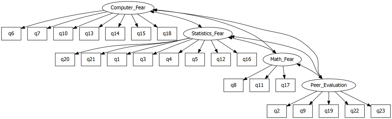
CFA For Anxiety Data
You can see here that I have constructed what is called a measurement model for the items in the anxiety questionnaire. This model is based on the factor analysis we just conducted. CFA is simply the way we test whether this model is a good fit to the data, does this factor structure correspond with the correlations between the items.
Now hopefully you are beginning to see the symmetry between path analysis and CFA in terms of the structural equation model. When we say how well the model fit, what we are saying is does the covariance matrix for the model approximate the covariance matrix for the data. Just like we did last week. The principal is exactly the same!
Only this time, we are testing a model with latent variables, which capture the common variances among the items. If the model fits well, that is to say the covariance matrices are more or less the same, then that is good evidence that the items indeed belong in their latent variable clusters. If the model does not fit well - there is a problem with our measurement.
There is an important advantage of modeling variables this way: latent variables are measured without error. That contain the common variance of the items therefore do not contain any unique or error variance. We have solved the problem of imperfect measurement!
Building a CFA model
To define our CFA model for the anxiety data we are going to use lavaan. As noted last week, to define models in lavaan you must specify the relationships between variables in a text format. A full guide to this lavaan model syntax is available on the lavaan project website.
For CFA models, like path models, the format is fairly simple, and resembles a series of linear models, written over several lines.
In the model below there are four latent variables, computer fear, statistics fear, math fear, and peer evaluation. The latent variable names are followed by =~ which means ‘is manifested by’, and then the observed variables, our items for the latent variable, are listed, separated by the + symbol.
cfa.model <- "
computerFear =~ Q06 + Q07 + Q10 + Q13 + Q14 + Q15 + Q18
statisticsFear=~ Q01 + Q03 + Q04 + Q05 + Q12 + Q16 + Q20 + Q21
mathFear =~ Q08 + Q11 + Q17
peerEvaluation =~ Q02 + Q09 + Q19 + Q22 + Q23
"
Note that we have saved our model specification in a variable named cfa.model. Just like last week for path analysis.
The special symbols in the lavaan syntax used for latent varianbles in CFA models is =~ where the latent variable is listed before and the items listed after.
Testing the CFA Model
To run the analysis we pass the model specification and the data to the cfa() function. Again, just like last week:
# Recode that reverse item
#anxiety.cor$Q03 <- car::recode(anxiety.cor$Q03, "1=5; 2=4; 3=3; 4=2; 5=1")

# Fit the model
cfa.fit <- cfa(cfa.model, data=anxiety.cor)
summary(cfa.fit, fit.measures=TRUE, standardized=TRUE)
## lavaan 0.6-7 ended normally after 55 iterations
##
## Estimator ML
## Optimization method NLMINB
## Number of free parameters 52
##
## Number of observations 2571
##
## Model Test User Model:
##
## Test statistic 2273.274
## Degrees of freedom 224
## P-value (Chi-square) 0.000
##
## Model Test Baseline Model:
##
## Test statistic 19406.199
## Degrees of freedom 253
## P-value 0.000
##
## User Model versus Baseline Model:
##
## Comparative Fit Index (CFI) 0.893
## Tucker-Lewis Index (TLI) 0.879
##
## Loglikelihood and Information Criteria:
##
## Loglikelihood user model (H0) -74281.008
## Loglikelihood unrestricted model (H1) -73144.371
##
## Akaike (AIC) 148666.015
## Bayesian (BIC) 148970.322
## Sample-size adjusted Bayesian (BIC) 148805.103
##
## Root Mean Square Error of Approximation:
##
## RMSEA 0.060
## 90 Percent confidence interval - lower 0.057
## 90 Percent confidence interval - upper 0.062
## P-value RMSEA <= 0.05 0.000
##
## Standardized Root Mean Square Residual:
##
## SRMR 0.047
##
## Parameter Estimates:
##
## Standard errors Standard
## Information Expected
## Information saturated (h1) model Structured
##
## Latent Variables:
## Estimate Std.Err z-value P(>|z|) Std.lv Std.all
## computerFear =~
## Q06 1.000 0.709 0.632
## Q07 1.088 0.037 29.148 0.000 0.771 0.700
## Q10 0.533 0.028 19.384 0.000 0.378 0.431
## Q13 0.922 0.032 28.807 0.000 0.654 0.689
## Q14 0.933 0.033 27.935 0.000 0.661 0.662
## Q15 0.798 0.033 24.384 0.000 0.566 0.560
## Q18 1.094 0.036 30.283 0.000 0.776 0.737
## statisticsFear =~
## Q01 1.000 0.490 0.592
## Q03 -1.367 0.054 -25.302 0.000 -0.670 -0.623
## Q04 1.239 0.048 25.792 0.000 0.607 0.640
## Q05 1.086 0.047 23.087 0.000 0.532 0.552
## Q12 1.236 0.047 26.391 0.000 0.606 0.661
## Q16 1.267 0.047 26.861 0.000 0.621 0.678
## Q20 0.936 0.048 19.306 0.000 0.458 0.443
## Q21 1.323 0.050 26.321 0.000 0.648 0.658
## mathFear =~
## Q08 1.000 0.661 0.758
## Q11 1.064 0.029 36.866 0.000 0.703 0.799
## Q17 1.029 0.029 35.926 0.000 0.680 0.770
## peerEvaluation =~
## Q02 1.000 0.410 0.482
## Q09 1.630 0.106 15.384 0.000 0.669 0.529
## Q19 1.407 0.092 15.315 0.000 0.577 0.524
## Q22 1.206 0.083 14.617 0.000 0.495 0.475
## Q23 0.696 0.069 10.029 0.000 0.285 0.273
##
## Covariances:
## Estimate Std.Err z-value P(>|z|) Std.lv Std.all
## computerFear ~~
## statisticsFear 0.291 0.015 19.844 0.000 0.837 0.837
## mathFear 0.304 0.016 19.525 0.000 0.648 0.648
## peerEvaluation -0.147 0.011 -13.030 0.000 -0.507 -0.507
## statisticsFear ~~
## mathFear 0.220 0.011 19.381 0.000 0.679 0.679
## peerEvaluation -0.115 0.008 -13.598 0.000 -0.571 -0.571
## mathFear ~~
## peerEvaluation -0.079 0.009 -9.097 0.000 -0.290 -0.290
##
## Variances:
## Estimate Std.Err z-value P(>|z|) Std.lv Std.all
## .Q06 0.756 0.023 32.355 0.000 0.756 0.601
## .Q07 0.620 0.020 30.777 0.000 0.620 0.510
## .Q10 0.626 0.018 34.662 0.000 0.626 0.814
## .Q13 0.472 0.015 31.075 0.000 0.472 0.525
## .Q14 0.559 0.018 31.732 0.000 0.559 0.561
## .Q15 0.699 0.021 33.451 0.000 0.699 0.686
## .Q18 0.507 0.017 29.560 0.000 0.507 0.457
## .Q01 0.445 0.013 33.077 0.000 0.445 0.650
## .Q03 0.707 0.022 32.578 0.000 0.707 0.612
## .Q04 0.531 0.016 32.272 0.000 0.531 0.591
## .Q05 0.647 0.019 33.603 0.000 0.647 0.696
## .Q12 0.473 0.015 31.840 0.000 0.473 0.563
## .Q16 0.453 0.014 31.447 0.000 0.453 0.540
## .Q20 0.862 0.025 34.605 0.000 0.862 0.804
## .Q21 0.549 0.017 31.894 0.000 0.549 0.566
## .Q08 0.324 0.012 26.281 0.000 0.324 0.426
## .Q11 0.280 0.012 23.292 0.000 0.280 0.362
## .Q17 0.318 0.012 25.504 0.000 0.318 0.408
## .Q02 0.556 0.019 29.910 0.000 0.556 0.768
## .Q09 1.148 0.041 28.167 0.000 1.148 0.720
## .Q19 0.880 0.031 28.390 0.000 0.880 0.726
## .Q22 0.838 0.028 30.118 0.000 0.838 0.774
## .Q23 1.008 0.029 34.290 0.000 1.008 0.925
## computerFear 0.503 0.030 16.856 0.000 1.000 1.000
## statisticsFear 0.240 0.015 15.556 0.000 1.000 1.000
## mathFear 0.437 0.021 20.852 0.000 1.000 1.000
## peerEvaluation 0.168 0.017 10.188 0.000 1.000 1.000The output has four parts:
Model fit. The extent to which the model implied covariance matrix approximates the observed covariance matrix
Parameter estimates. The values in the first column are the unstandardised weights from the observed variables to the latent factors. The standardized wights are in the std.all column. We will inspect the standardized weights as they give us an interpretible metric for model diagnostics.
Factor covariances. In CFA the factors are correlated with each other to account for the interrelation of the factors that make up the underlying data. These values are the covariances between the latent factors. The values in the std.all column are the correlation coefficients between the latent variables (standardized covariance)
Error variances. These values are the estimates of each item’s error variance (i.e., what is left over after the common variance has been subtracted out).
What can we say from this output? Well, the CFI and TLI are our first areas of concern. They are below the .90 threshold that we discussed last week. The RMSEA and the SRMR look good though. Both are below .10.
When we take a look at the standardized factor loadings for the latent variables, we see a few issues. There is one item here with low loading on its hypothesised factor (Q23 of Peer Evaluation; “If I am good at statistics, people will think I’m a nerd”). It had a standardised loading of 0.27 One rule of thumb is that factor loadings < .40 are weak and factor loadings > .60 are strong (Garson, 2010). This is a very weak loading so we should remove the item and respecify the model.
We also see a negative factor loading here for Q03 on the statistics fear latent variable. When we look at the questionnaire, it is evident that Q03 is a bit ambiguous and should be reverse coded (“standard deviations excite me”). Again, given the ambiguity and negative loading, we need to remove it and respecify the model.
# Model respecifcation removing Q03 and Q23

cfa.model2 <- "
computerFear =~ Q06 + Q07 + Q10 + Q13 + Q14 + Q15 + Q18
statisticsFear=~ Q01 + Q04 + Q05 + Q12 + Q16 + Q20 + Q21
mathFear =~ Q08 + Q11 + Q17
peerEvaluation =~ Q02 + Q09 + Q19 + Q22
"

# Fit the respecified model

cfa.fit2 <- cfa(cfa.model2, data=anxiety.cor)
summary(cfa.fit2, fit.measures=TRUE, standardized=TRUE)
## lavaan 0.6-7 ended normally after 55 iterations
##
## Estimator ML
## Optimization method NLMINB
## Number of free parameters 48
##
## Number of observations 2571
##
## Model Test User Model:
##
## Test statistic 1918.901
## Degrees of freedom 183
## P-value (Chi-square) 0.000
##
## Model Test Baseline Model:
##
## Test statistic 17885.770
## Degrees of freedom 210
## P-value 0.000
##
## User Model versus Baseline Model:
##
## Comparative Fit Index (CFI) 0.902
## Tucker-Lewis Index (TLI) 0.887
##
## Loglikelihood and Information Criteria:
##
## Loglikelihood user model (H0) -67272.844
## Loglikelihood unrestricted model (H1) -66313.394
##
## Akaike (AIC) 134641.688
## Bayesian (BIC) 134922.586
## Sample-size adjusted Bayesian (BIC) 134770.077
##
## Root Mean Square Error of Approximation:
##
## RMSEA 0.061
## 90 Percent confidence interval - lower 0.058
## 90 Percent confidence interval - upper 0.063
## P-value RMSEA <= 0.05 0.000
##
## Standardized Root Mean Square Residual:
##
## SRMR 0.046
##
## Parameter Estimates:
##
## Standard errors Standard
## Information Expected
## Information saturated (h1) model Structured
##
## Latent Variables:
## Estimate Std.Err z-value P(>|z|) Std.lv Std.all
## computerFear =~
## Q06 1.000 0.710 0.633
## Q07 1.085 0.037 29.137 0.000 0.770 0.699
## Q10 0.534 0.027 19.443 0.000 0.379 0.432
## Q13 0.924 0.032 28.901 0.000 0.655 0.691
## Q14 0.930 0.033 27.925 0.000 0.660 0.661
## Q15 0.797 0.033 24.412 0.000 0.566 0.561
## Q18 1.092 0.036 30.300 0.000 0.775 0.736
## statisticsFear =~
## Q01 1.000 0.498 0.601
## Q04 1.231 0.047 26.080 0.000 0.613 0.646
## Q05 1.085 0.046 23.398 0.000 0.540 0.560
## Q12 1.217 0.046 26.503 0.000 0.606 0.661
## Q16 1.249 0.046 27.012 0.000 0.622 0.679
## Q20 0.898 0.048 18.889 0.000 0.447 0.432
## Q21 1.297 0.049 26.347 0.000 0.645 0.656
## mathFear =~
## Q08 1.000 0.662 0.759
## Q11 1.061 0.029 36.840 0.000 0.702 0.798
## Q17 1.028 0.029 35.953 0.000 0.681 0.770
## peerEvaluation =~
## Q02 1.000 0.410 0.481
## Q09 1.598 0.108 14.739 0.000 0.655 0.518
## Q19 1.420 0.096 14.848 0.000 0.582 0.528
## Q22 1.169 0.084 13.946 0.000 0.479 0.460
##
## Covariances:
## Estimate Std.Err z-value P(>|z|) Std.lv Std.all
## computerFear ~~
## statisticsFear 0.297 0.015 19.956 0.000 0.840 0.840
## mathFear 0.305 0.016 19.540 0.000 0.648 0.648
## peerEvaluation -0.152 0.012 -13.026 0.000 -0.522 -0.522
## statisticsFear ~~
## mathFear 0.225 0.012 19.460 0.000 0.682 0.682
## peerEvaluation -0.109 0.008 -12.981 0.000 -0.537 -0.537
## mathFear ~~
## peerEvaluation -0.079 0.009 -8.940 0.000 -0.290 -0.290
##
## Variances:
## Estimate Std.Err z-value P(>|z|) Std.lv Std.all
## .Q06 0.755 0.023 32.341 0.000 0.755 0.600
## .Q07 0.622 0.020 30.817 0.000 0.622 0.512
## .Q10 0.625 0.018 34.654 0.000 0.625 0.813
## .Q13 0.470 0.015 31.022 0.000 0.470 0.522
## .Q14 0.561 0.018 31.758 0.000 0.561 0.563
## .Q15 0.698 0.021 33.448 0.000 0.698 0.686
## .Q18 0.508 0.017 29.583 0.000 0.508 0.458
## .Q01 0.438 0.013 32.625 0.000 0.438 0.639
## .Q04 0.524 0.016 31.747 0.000 0.524 0.582
## .Q05 0.639 0.019 33.257 0.000 0.639 0.687
## .Q12 0.473 0.015 31.407 0.000 0.473 0.563
## .Q16 0.452 0.015 30.941 0.000 0.452 0.539
## .Q20 0.872 0.025 34.557 0.000 0.872 0.814
## .Q21 0.553 0.018 31.537 0.000 0.553 0.570
## .Q08 0.323 0.012 26.204 0.000 0.323 0.424
## .Q11 0.282 0.012 23.361 0.000 0.282 0.364
## .Q17 0.318 0.012 25.450 0.000 0.318 0.407
## .Q02 0.556 0.019 29.367 0.000 0.556 0.768
## .Q09 1.166 0.042 27.918 0.000 1.166 0.731
## .Q19 0.874 0.032 27.487 0.000 0.874 0.721
## .Q22 0.853 0.028 30.085 0.000 0.853 0.788
## computerFear 0.504 0.030 16.881 0.000 1.000 1.000
## statisticsFear 0.248 0.016 15.752 0.000 1.000 1.000
## mathFear 0.438 0.021 20.877 0.000 1.000 1.000
## peerEvaluation 0.168 0.017 9.931 0.000 1.000 1.000Now we have CFI = .90, TLI .89, RMSEA = .06, and SRMR = .05. As well, all standardised factor loadings are > .40. That’s pretty good! Our anxiety questionnaire has successfully passed the EFA and CFA with four factors that fit the data adequately from the initial pool of 23 item items. Lets visualize that model with semPlot plotting the standardized factor loadings and covariances (correlations):
semPaths(cfa.fit2, "std")
We are done!
Activity: Holzinger and Swineford Factor Analysis
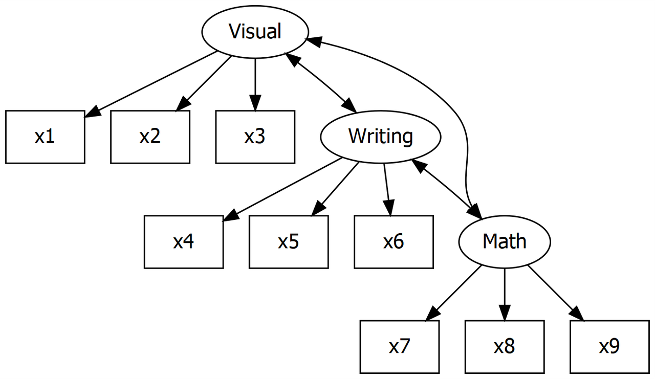
The classic Holzinger and Swineford (1939) study of mental ability consists of mental ability test scores of seventh- and eighth-grade children from two different schools (Pasteur and Grant-White).
In the original dataset, there are scores for 26 tests. However, a smaller subset with 9 variables is more widely used in the literature (for example in Joreskog’s 1969 paper, which also uses the 145 subjects from the Grant-White school only). These mental abilities are:
x1 Visual perception
x2 Cubes
x3 Lozenges
x4 Paragraph comprehension
x5 Sentence completion
x6 Word meaning
x7 Speeded addition
x8 Speeded counting of dots
x9 Speeded discrimination straight and curved capitals
Holzinger and Swineford thought that these abilities could be condensed into three latent abilities for visual skill, writing skill, and math skill:
Visual skill was hypothesized as a combination of x1, x2, and x3
Writing skill was hypothesized as a combination of x4, x5, and x6
Math skill was hypothesized as a combination of x7, x8, and x9
The CFA model looks like this:
Holzinger and Swineford Model of Mental Ability
Load data
Luckily, the Holzinger and Swineford dataset is a practice dataset contained in the lavaan package for CFA, so we don;t need to load it from the computer, we can load it from the package. Lets do that now:
mental <- lavaan::HolzingerSwineford1939
head(mental)
## id sex ageyr agemo school grade x1 x2 x3 x4 x5 x6
## 1 1 1 13 1 Pasteur 7 3.333333 7.75 0.375 2.333333 5.75 1.2857143
## 2 2 2 13 7 Pasteur 7 5.333333 5.25 2.125 1.666667 3.00 1.2857143
## 3 3 2 13 1 Pasteur 7 4.500000 5.25 1.875 1.000000 1.75 0.4285714
## 4 4 1 13 2 Pasteur 7 5.333333 7.75 3.000 2.666667 4.50 2.4285714
## 5 5 2 12 2 Pasteur 7 4.833333 4.75 0.875 2.666667 4.00 2.5714286
## 6 6 2 14 1 Pasteur 7 5.333333 5.00 2.250 1.000000 3.00 0.8571429
## x7 x8 x9
## 1 3.391304 5.75 6.361111
## 2 3.782609 6.25 7.916667
## 3 3.260870 3.90 4.416667
## 4 3.000000 5.30 4.861111
## 5 3.695652 6.30 5.916667
## 6 4.347826 6.65 7.500000You can see we have some demographic information and then the items that we are going to run CFA with to confirm the factor structure hypothesised by Holzinger and Swineford.
Lets do that now.
Build the CFA model
Write the script to build the model for three latent variables: visual, writing, and math. Dont forget to specify the latent variables with “=~”. Save the model object as “mental.model”
mental.model <- "
visual =~ x1 + x2 + x3
writing =~ x4 + x5 + x6
maths =~ x7 + x8 + x9
"
Fit the CFA Model
Now write the code to fit the CFA model to the data and save it as a new object called “mental.fit”. Then request the summary estiamtes:
# Fit the CFA model
mental.fit <- cfa(mental.model, data=mental)

# Summarise the fit
summary(mental.fit, fit.measures=TRUE, standardized=TRUE)
## lavaan 0.6-7 ended normally after 35 iterations
##
## Estimator ML
## Optimization method NLMINB
## Number of free parameters 21
##
## Number of observations 301
##
## Model Test User Model:
##
## Test statistic 85.306
## Degrees of freedom 24
## P-value (Chi-square) 0.000
##
## Model Test Baseline Model:
##
## Test statistic 918.852
## Degrees of freedom 36
## P-value 0.000
##
## User Model versus Baseline Model:
##
## Comparative Fit Index (CFI) 0.931
## Tucker-Lewis Index (TLI) 0.896
##
## Loglikelihood and Information Criteria:
##
## Loglikelihood user model (H0) -3737.745
## Loglikelihood unrestricted model (H1) -3695.092
##
## Akaike (AIC) 7517.490
## Bayesian (BIC) 7595.339
## Sample-size adjusted Bayesian (BIC) 7528.739
##
## Root Mean Square Error of Approximation:
##
## RMSEA 0.092
## 90 Percent confidence interval - lower 0.071
## 90 Percent confidence interval - upper 0.114
## P-value RMSEA <= 0.05 0.001
##
## Standardized Root Mean Square Residual:
##
## SRMR 0.065
##
## Parameter Estimates:
##
## Standard errors Standard
## Information Expected
## Information saturated (h1) model Structured
##
## Latent Variables:
## Estimate Std.Err z-value P(>|z|) Std.lv Std.all
## visual =~
## x1 1.000 0.900 0.772
## x2 0.554 0.100 5.554 0.000 0.498 0.424
## x3 0.729 0.109 6.685 0.000 0.656 0.581
## writing =~
## x4 1.000 0.990 0.852
## x5 1.113 0.065 17.014 0.000 1.102 0.855
## x6 0.926 0.055 16.703 0.000 0.917 0.838
## maths =~
## x7 1.000 0.619 0.570
## x8 1.180 0.165 7.152 0.000 0.731 0.723
## x9 1.082 0.151 7.155 0.000 0.670 0.665
##
## Covariances:
## Estimate Std.Err z-value P(>|z|) Std.lv Std.all
## visual ~~
## writing 0.408 0.074 5.552 0.000 0.459 0.459
## maths 0.262 0.056 4.660 0.000 0.471 0.471
## writing ~~
## maths 0.173 0.049 3.518 0.000 0.283 0.283
##
## Variances:
## Estimate Std.Err z-value P(>|z|) Std.lv Std.all
## .x1 0.549 0.114 4.833 0.000 0.549 0.404
## .x2 1.134 0.102 11.146 0.000 1.134 0.821
## .x3 0.844 0.091 9.317 0.000 0.844 0.662
## .x4 0.371 0.048 7.779 0.000 0.371 0.275
## .x5 0.446 0.058 7.642 0.000 0.446 0.269
## .x6 0.356 0.043 8.277 0.000 0.356 0.298
## .x7 0.799 0.081 9.823 0.000 0.799 0.676
## .x8 0.488 0.074 6.573 0.000 0.488 0.477
## .x9 0.566 0.071 8.003 0.000 0.566 0.558
## visual 0.809 0.145 5.564 0.000 1.000 1.000
## writing 0.979 0.112 8.737 0.000 1.000 1.000
## maths 0.384 0.086 4.451 0.000 1.000 1.000Summarize the key fit indexes for this model. Are they indicative of adequate fit?
Do the items loading well on their respective latent variables?
How are the factors correlated with each other?
Visulaise the CFA
Finally, write the code to visualize the CFA model with the standardised estimates plotted. Dont forget to use semPaths
semPaths(mental.fit, "std")
Nice job!
– This post covers my notes of Exploratory Factor Analysis which draw some help from the book “Discovering Statistics using R (2012)” by Andy Field. Some code and text come from the book. For those parts, credit goes to him.