Latent Variable Structural Equation Modeling (LT4)
Preliminaries
library(readr)
library(lavaan)
library(semPlot)
Introduction
This week we are going to combine our understanding of path analysis and confirmatory factor analysis to finish this section of the course with full latent variable strucutral equation modeling. Before we begin, though. Let’s recap where we are before we get into SEM analysis.
The Roots of Structural Equation Modeling
To date we have covered all the core concepts needed to understand and apply latent variable SEM. It is is complex analysis, but you have all the building blocks.
Last week, we looked at factor analytic techniques that test the assumption of a general factor of underlying a set of items (typically questionnaire items). This technique allows us to reduce a large number of variables to a smaller number of underlying constructs that are represented by unobserved or latent variables. We can test the fit of this measurement strucutre with confirmatory factor analysis, as we sw.
We also saw last year with the general linear model a technique called multiple regression that allowed estimating the relation between two constructs while controlling for the otherwise biasing effects of confounding variables.
Finally, when we looked at path analysis, we saw Wright’s tracing rules and path analytic techniques in which causal relations between various variables could be estimated at the same time. Below is an overview of these thre analyses, using simplified path diagram visualizations that are often used to depict SEMs.
These are the basic building blocks of SEM.

A graphical depiction of three major statistical techniques
Latent Variable Structural Equation Modeling
Based on these three techniques, statisticians started to think about some of the first SEM related techniques, which would allow researchers to break out of the boundaries of traditional statistical methods.
It was a stroke of genius. They worked out a way to merge the logic of factor analysis, multiple regression, and path analysis. This yielded the unifying, more general framework of whats called covariance structure modeling, which is the core method underlying the SEM framework.
Recall from path analysis that covariance structure modeling is a method that got its name because instead of modeling all individual data points of a dataset, one takes only the variables’ variances and covariances (relationships).
To visualize this technique, a “full” latent variable structural equation model is depicted below. Full means that the model has measurement parts and a structural part. The model combines aspects of all three mentioned classical statistical approaches.
In the measurement parts of the model, the outer model, puts the factor structure of the psychological constructs into latent variables. This is the same as what we do with confirmatory factor analysis.
The structural part of the model, the inner model, depicts how these latent psychological constructs relate to each other. Here, structures similar to multiple regression and path analysis are modeled.
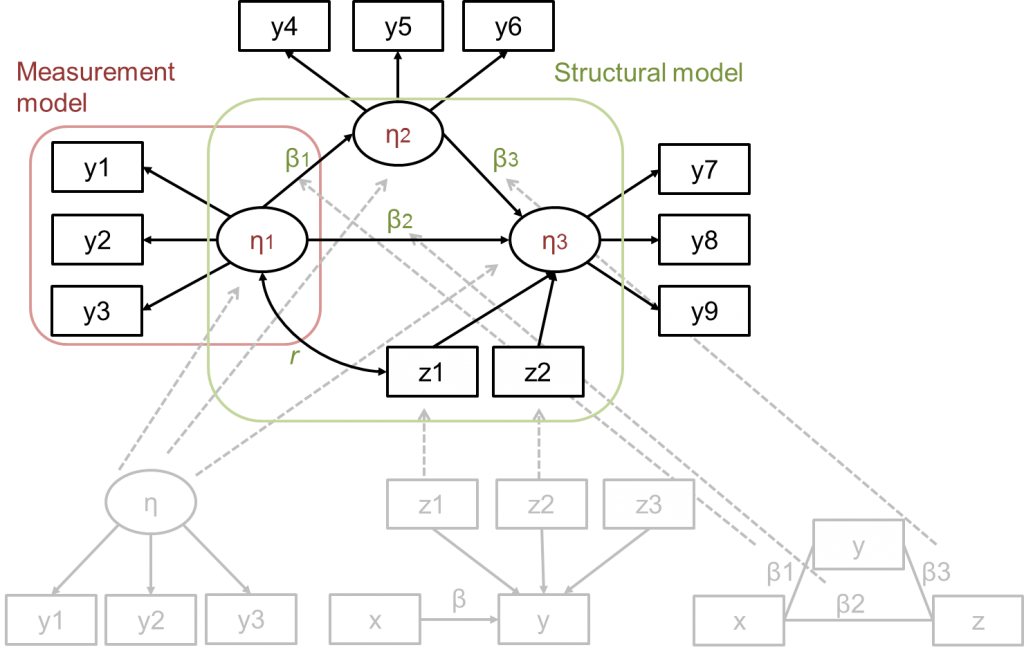
A depiction of a “full” structural equation model, including three measurement parts (one entangled in red) and a structural part (entangled in green
By combining the measurement model and structural model, we can both test the adequacy of our measurement (confirmatory factor analysis) and the causal relationships between our latent variables. Pretty neat!
The typical approach to this type of analysis is to test the measurement model first and then test the full structural model second (Anderson & Gerbin, 1988). We will look at these steps today.
Latent Variables: Chanting away measurement error
There are many advantages to SEM, but arguably the biggest is that it permits tests of relationships in the absence of measurement error. This is crucial because an assumption of regression analysis is that variables are measured without error.
Psychological characteristics are not directly measurable. We can ask people questions, we can measure their heart rate or brain activity, we can observe them in social interactions, but the resulting data do not directly tell us about people’s psychological characteristics.
Rather, we assume that our data relate to people’s psychological characteristics in specific ways that we try to model. In SEM, we do this by assuming that various variables correlate because they all indicate the level of the same psychological construct.
For example, in the assessment of creativity, people are often asked to suggest many novel and useful ideas about what to do with everyday objects such as a can, a car tire, or a brick (e.g. Benedek et al., 2014). We can count how many ideas people come up with for each of these items. How should we use the resulting numbers to determine how creative people are? The statistician answer to this question is the latent variable, the idea of which is depicted below.
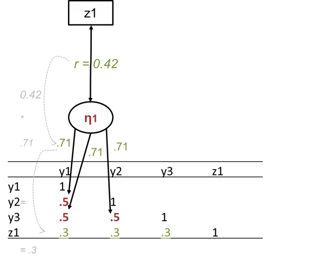
Depiction of a latent variable (η1) in SEM and how it represents correlations between indicators (y1–y3) and their relations with other variables (z1)
Above, a covariance matrix is depicted which shows that number of novel ideas is positively correlated across the three items (variables y1–y3). The more ideas people have for the can, the more ideas they tend to have as well for what to do with the car tire and the brick.
Why is this so? The creativity researcher’s assumption is, surprise surprise, because some people are more creative than others! From a psychological point of view, this assumption entails that people’s creativity is the psychological construct underlying their ideas on all three items.
Translating this into statistics, creativity is a latent variable that explains the correlations between the three items because it caused the variation underlying them. In the figure, this is indicated by arrows pointing from the latent variable representing creativity toward the variables representing people’s number of ideas on the three items.
Now, let’s see what it means to get rid of measurement error. In the correlation matrix there is also the variable z1, which represents people’s scores on a questionnaire that assesses openness. People’s openness for new experiences is positively correlated with their creativity. That is, being open might free people’s minds, and free minds might be open!
Also in the correlation matrix we see that the three creativity items show correlations of .3 with z1, the openness scores. In SEM, instead of modeling all of these three correlations, we sum up the items’ variance that represents creativity into a latent variable, η1. In this latent variable, all the variance that the three items share is represented (i.e., the common variance).
All the variance that the items do not share is assumed to be measurement error, which does not represent people’s creativity but rather assessment artifacts and randomness, and is thus left out of the latent variable. This can be seen in the three paths from the η1 variable to the y variables. These paths are factor loadings that show how strongly each item represents the construct that it is supposed to measure, in our case creativity. The factor loadings are all .71, which is lower than 1, indicating that only parts of the y variables’ variances go into the latent variable.
Below, there is a depiction of how measurement error variance is cut out of the indicator variables and only the share of variance which supposedly really represents creativity goes into the latent variable.
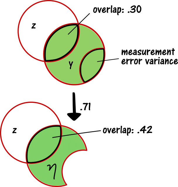
A variance cake illustration of the process of creating a latent variable
The initial correlation between any of the y variables and z is .30. This is represented as an overlap in the y and z variables’ variances in the upper part of the figure.
In the latent variable, only a part of any of the y variables’ variances is represented. However, the overlap in variance with the z variable is still the same. Crucially, the three y variables’ correlations with the z variable are now all represented by the latent variables’ correlation with the z variable.
However, for the latter two variables, the proportion of overlapping variance is larger (i.e., the relationship is greater). As a result, the correlation that the latent variable has with z1 is estimated to be .42. This is higher than the three y-variables’ individual correlation estimates with the z1 variable, because it is corrected for measurement error, by just cutting it out of the variance cake.
This is the reason why you can get rid of measurement error by using SEM. This might look like magic, but it is not; it is a strong theory about a measured construct that has been translated into a SEM.
Estimation
Estimating SEMs, like path analysis, consists of finding a set of parameters that fits the data best. For complex SEMs this is achieved by iterative algorithms, typically a maximum likelihood estimator, as we saw in the path analysis session (this is why SEM analyses do not have intercepts, the estimators and SEs are estimated by maximum likelihood, which we saw last year in logistic regression)
Put simply, though, the estimation of SEMs can be well understood by applying Wright’s path tracing rules - just like in the path analysis session. Even though the estimators are quite complex in big models, the underlying principal is not too complicated!
To sum up the estimation, lets go back to the creativity example. The correlations of the three creativity test items with each other are represented in the estimates of the factor loadings, and all three of the items’ correlations with the z variable are represented in the latent variables’ estimated correlation with the z variable, which is corrected for measurement error through the factor loadings.
Awesome. Let’s go ahead and run the analyses!
Activity: The Data
To apply latent variable SEM, we are going to use data from a paper I published a few years back:
Curran, T. (2018). Parental conditional regard and the development of perfectionism in adolescent athletes: the mediating role of competence contingent self-worth. Sport, Exercise, and Performance Psychology, 7(3), 284.
This paper looked to examine the role of parent conditional regard on young people’ perfectionism through the mediated pathway of contingent self-worth in 148 young athletes aged between 12 and 18.
Lets load this data now:
parent <- read_csv("C:/Users/CURRANT/Dropbox/Work/LSE/PB230/LT4/Workshop/parent.csv")##
## -- Column specification --------------------------------------------
## cols(
## ID = col_double(),
## Gender = col_double(),
## Age_Child = col_double(),
## csw1 = col_double(),
## csw2 = col_double(),
## csw3 = col_double(),
## csw4 = col_double(),
## csw5 = col_double(),
## sop = col_double(),
## spp = col_double(),
## ps = col_double(),
## doa = col_double(),
## com = col_double(),
## cr1 = col_double(),
## cr2 = col_double(),
## cr3 = col_double(),
## cr4 = col_double(),
## cr5 = col_double()
## )head(parent)## # A tibble: 6 x 18
## ID Gender Age_Child csw1 csw2 csw3 csw4 csw5 sop spp ps doa
## <dbl> <dbl> <dbl> <dbl> <dbl> <dbl> <dbl> <dbl> <dbl> <dbl> <dbl> <dbl>
## 1 41 2 13 5 5 5 6 4 6.2 5.6 4.57 2.67
## 2 106 2 15 6 7 6 6 6 5.8 6.6 4.14 3.17
## 3 107 1 15 6 6 6 6 2 5.8 6.2 3.29 3.5
## 4 29 1 17 4 6 2 4 4 5 3.6 2.86 2
## 5 115 1 14 5 7 6 6 1 2.98 4.6 3.14 2.33
## 6 16 2 15 6 7 7 7 6 6 6.2 4.43 2.5
## # ... with 6 more variables: com <dbl>, cr1 <dbl>, cr2 <dbl>, cr3 <dbl>,
## # cr4 <dbl>, cr5 <dbl>In the parent data are fifteen variables that comprise four latent variables:
Latent Variable 1: Parent Conditional Regard. Conditional regard is a controlling parental style whereby parents withhold love and affection when children have performed badly. It was measured with 5 items from the Parental Conditional Negative Regard Scale (Assor & Tal, 2012). The instrument assesses the degree to which children perceive their mother and father to be conditionally regarding separately and then scores are combined. The items were adapted slightly to measure parental conditional regard in the sport domain (e.g., “When I perform badly in sport, my mother/father stops giving me attention for a while”). The scale is rated on a 7-point Likert scale ranging from 1 (strongly disagree) to 7 (strongly agree).
Items for the latent parent conditional regard variable in the dataset: cr1, cr2, cr3, cr4, cr5
Latent Variable 2: Contingent Self-Worth. Contingent self-worth is self-worth that is dependent (contingent) on performances. If someone has high contingent self-worth then their self-worth is strognly tied to their performances and they only feel good about themselves when they have performed well. It is measured with 5 items from the Contingencies of Self-Worth Scale (Crocker, Luhtanen, Cooper, & Bouvrette, 2003). To anchor responses in the correct domain, the items were adapted to measure competence contingent self-worth in sport (e.g., “I feel better about myself when I know I’m doing well in sport.”). Participants provide ratings of agreement on scales ranging from 1 (strongly disagree) to 7 (strongly agree).
Items for the latent contingent self-worth variable in the dataset: csw1, csw2, csw3, csw4, csw5
Latent Variable 3: Perfectionistic Strivings. Perfectionistic strivings are the dimension of perfectionism that come from within (i.e., high self-set goals and expectations). Two measures were used as indicators of perfectionistic strivings in this study. They were the mean of the five item self-oriented perfectionism subscale of the HF-MPS (e.g., “One of my goals is to be perfect in everything I do.”) and the mean of the seven-item personal standards subscale of the F-MPS (e.g., “I hate being less than the best at things in my sport”). The HF-MPS has a 1-5 Likert scale and the F-MPS has a 1-7 Likert scale.
Items for the latent perfectionistic strivings variable in the dataset: sop and ps
Latent Variable 3: Perfectionistic Concerns. Perfectionistic concerns are the dimension of perfectionism that come from concerns of others (i.e., others high expectation and doubts about actions). Three measures were used as indicators of perfectionistic concerns in this study. They were the mean of the five item socially prescribed perfectionism subscale of the HF-MPS (e.g., “People expect nothing less than perfection from me.”), the mean of the eight-item concern over mistakes subscale of the F-MPS (e.g., “If I fail in competition I feel like a failure as a person”), and the mean of the six-item doubts about actions subscale from the F-MPS (e.g., “I usually feel unsure about the adequacy of my pre-competition practices”). The HF-MPS has a 1-5 Likert scale and the F-MPS has a 1-7 Likert scale.
Items for the latent perfectionistic strivings variable in the dataset: spp, com, and doa
The model to be tested is seen below. All relationships were hypothesized to be positive:

Hypothesised SEM Model
I have cleaned and screened all the data in the parents dataset, so we are all ready to go!
Step 1: Testing the Measurement Model (CFA)
Typically the first step in structural equation modeling is to establish what’s called a “measurement model”, a model which includes all of your observed variables that are going to be represented with latent variables.
Constructing a measurement model allows to determine model fit related to the measurement portion of your model. This is exactly the same analysis as CFA last week, except this time we are checking the measurement of your causal model (rather than the factor structure of a new questionnaire). By running CFA on our model first, we can more precisely know where any model misfit is and make necessary adjustments. But, provided the variables measure what they are supposed to be measuring, we should have few issues.
Below is the depicition of our measurement model for the parent data:

CFA Model for Parent Data
Note there are no causal paths here from our hypothesized model above, just covarainces between the latent variables. We are not interested in testing the adequecy of the hypothesised model yet. Simply, we want to know: is the measurement good? Do the items belong to their intended latent variables?
To test this we will build the CFA model in laavan, just like we have been doing to date.
Recall that the lavaan syntax used for latent variables in CFA models is “=~” where the latent variable is listed before and the items listed after. Also recall that we fix the first item to 1 so that a one unit change in the latent variable is interpreted as 1 unit unit change in the scale of the that item.
Lets build the measurement model now, saving the object as measurement.model.
measurement.model <- "
conditional_regard =~ 1*cr1 + cr2 + cr3 + cr4 + cr5
contingent_self_worth =~ 1*csw1 + csw2 + csw3 + csw4 + csw5
perfectionistic_strivings =~ 1*sop + ps
perfectionistic_concerns =~ 1*spp + com + doa
"
Great, now lets fit that measurement model and request the fit indexes and model parameters.
measurement.model.fit <- cfa(measurement.model, data=parent)
summary(measurement.model.fit, fit.measures=TRUE, standardized=TRUE)
## lavaan 0.6-7 ended normally after 55 iterations
##
## Estimator ML
## Optimization method NLMINB
## Number of free parameters 36
##
## Number of observations 149
##
## Model Test User Model:
##
## Test statistic 189.839
## Degrees of freedom 84
## P-value (Chi-square) 0.000
##
## Model Test Baseline Model:
##
## Test statistic 1454.853
## Degrees of freedom 105
## P-value 0.000
##
## User Model versus Baseline Model:
##
## Comparative Fit Index (CFI) 0.922
## Tucker-Lewis Index (TLI) 0.902
##
## Loglikelihood and Information Criteria:
##
## Loglikelihood user model (H0) -2742.533
## Loglikelihood unrestricted model (H1) -2647.614
##
## Akaike (AIC) 5557.067
## Bayesian (BIC) 5665.209
## Sample-size adjusted Bayesian (BIC) 5551.279
##
## Root Mean Square Error of Approximation:
##
## RMSEA 0.092
## 90 Percent confidence interval - lower 0.075
## 90 Percent confidence interval - upper 0.109
## P-value RMSEA <= 0.05 0.000
##
## Standardized Root Mean Square Residual:
##
## SRMR 0.076
##
## Parameter Estimates:
##
## Standard errors Standard
## Information Expected
## Information saturated (h1) model Structured
##
## Latent Variables:
## Estimate Std.Err z-value P(>|z|) Std.lv
## conditional_regard =~
## cr1 1.000 1.117
## cr2 0.941 0.057 16.456 0.000 1.052
## cr3 1.038 0.059 17.726 0.000 1.159
## cr4 0.753 0.054 13.837 0.000 0.841
## cr5 0.884 0.054 16.317 0.000 0.987
## contingent_self_worth =~
## csw1 1.000 0.613
## csw2 0.948 0.219 4.328 0.000 0.581
## csw3 1.637 0.312 5.253 0.000 1.003
## csw4 2.013 0.361 5.569 0.000 1.233
## csw5 1.019 0.273 3.732 0.000 0.624
## perfectionistic_strivings =~
## sop 1.000 0.621
## ps 0.953 0.155 6.167 0.000 0.592
## perfectionistic_concerns =~
## spp 1.000 0.783
## com 0.935 0.128 7.318 0.000 0.732
## doa 0.326 0.072 4.550 0.000 0.255
## Std.all
##
## 0.852
## 0.933
## 0.966
## 0.854
## 0.929
##
## 0.514
## 0.480
## 0.666
## 0.783
## 0.391
##
## 0.698
## 0.848
##
## 0.634
## 0.868
## 0.428
##
## Covariances:
## Estimate Std.Err z-value P(>|z|) Std.lv
## conditional_regard ~~
## cntngnt_slf_wr 0.148 0.070 2.112 0.035 0.217
## prfctnstc_strv 0.088 0.067 1.324 0.186 0.127
## prfctnstc_cncr 0.414 0.102 4.076 0.000 0.474
## contingent_self_worth ~~
## prfctnstc_strv 0.213 0.060 3.558 0.000 0.560
## prfctnstc_cncr 0.338 0.085 3.967 0.000 0.705
## perfectionistic_strivings ~~
## prfctnstc_cncr 0.303 0.075 4.049 0.000 0.623
## Std.all
##
## 0.217
## 0.127
## 0.474
##
## 0.560
## 0.705
##
## 0.623
##
## Variances:
## Estimate Std.Err z-value P(>|z|) Std.lv Std.all
## .cr1 0.473 0.060 7.909 0.000 0.473 0.275
## .cr2 0.166 0.025 6.715 0.000 0.166 0.130
## .cr3 0.097 0.020 4.766 0.000 0.097 0.068
## .cr4 0.263 0.033 7.894 0.000 0.263 0.271
## .cr5 0.155 0.023 6.835 0.000 0.155 0.137
## .csw1 1.045 0.133 7.841 0.000 1.045 0.736
## .csw2 1.128 0.141 7.976 0.000 1.128 0.770
## .csw3 1.262 0.185 6.821 0.000 1.262 0.556
## .csw4 0.960 0.189 5.080 0.000 0.960 0.387
## .csw5 2.163 0.263 8.240 0.000 2.163 0.847
## .sop 0.407 0.071 5.695 0.000 0.407 0.513
## .ps 0.137 0.051 2.666 0.008 0.137 0.281
## .spp 0.911 0.123 7.437 0.000 0.911 0.598
## .com 0.175 0.054 3.251 0.001 0.175 0.246
## .doa 0.291 0.035 8.263 0.000 0.291 0.817
## conditinl_rgrd 1.249 0.193 6.461 0.000 1.000 1.000
## cntngnt_slf_wr 0.375 0.125 3.012 0.003 1.000 1.000
## prfctnstc_strv 0.386 0.095 4.046 0.000 1.000 1.000
## prfctnstc_cncr 0.613 0.155 3.964 0.000 1.000 1.000What can we see from this analysis? We have CFI = .92, TLI .90, RMSEA = .09, and SRMR = .08. Thats pretty good! All of these fit indexes meet the thresholds for adequate fit that we have discussing (i.e., TLI & CFI > .90; RMSEA and SRMR < .10)
As well, all but one standardised factor loading is > .40. That’s also pretty good! We can take that one item out, csw5, if we want. But the fit is fine so it is also justifiable to leave it in. We will leave it in here.
Error Free Correlations
The other thing of note in this output are the standardised covariances between the latent variables, listed under covariances. These are the error free correlation coefficients, equivalent to Pearson’s r between the latent variables. With these correlations, we could create a matrix of error free correlations (error free because they reflect the correlation between latent variables, which are measured without error):
Standardised Covariances Between Latent Variables (Error-Free Correlations)
Composite Reliability
Also here we can calculate whats called the composite reliability of our latent variables, which is a bit like Cronbach’s alpha but calculated from the factor loadings not split-half correlations. Although it’s not perfect, composite reliability takes care of many inappropriate assumptions that measures like Cronbach’s alpha make (including that a higher number of items means greater reliability).
Composite reliability is calculated as:
sum(sl)^2 / (sum(sl)^2 + sum(re))
where sum(s1) is the sum of the standardsied factor loadings and sum(re) is the sum of the residual variances (i.e., 1-s1^2). Let’s quickly calculate the composite reliability of parent conditional regard:
# save standardised factor loadings in object s1
sl <- standardizedSolution(measurement.model.fit)

# extract from s1 standardised estimates (est.std) form only parent conditional regard
sl <- sl$est.std[sl$lhs == "conditional_regard"]

# calculate the residual variances
re <- 1 - sl^2

# calculate the composite reliability
sum(sl)^2 / (sum(sl)^2 + sum(re))
## [1] 0.9182011We can see that the composite estimate of reliability is .92, within errors of rounding to those reported in the paper (I calculated the composite reliability by hand in the paper). We can run this code for all latent variables or there is a useful website, which will do the calculations for you from the standardised factor loadings here: http://www.thestatisticalmind.com/calculators/comprel/composite_reliability.htm
Visulaising the CFA
As always, we can visualise the model being tested using semPaths:
semPaths(measurement.model.fit, "std")
And we are done for CFA!
How its written
The measurement model consisted of four inter-correlated latent variables. The five mother and five father conditional regard items were combined and used as the measured variables for the parental conditional regard factor (five indicators). Items were also used as the measured variables for the competence contingent self-worth factor (five indicators). For the perfectionism dimensions, subscales were used as measured variables for perfectionistic strivings (two indicators; self-oriented perfectionism and personal standards) and perfectionistic concerns (three indicators; socially prescribed perfectionism, doubts about actions, and concern over mistakes).
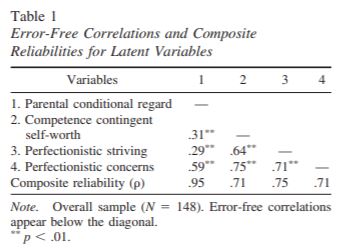
All standardised factor loadings for the measured variables on their latent factors were significant (parental conditional regard β range = .85 to .97; competence contingent self-worth β range = .39 to .78; perfectionistic strivings β range = .70 & .85; perfectionistic concerns β range = .43 to .87). Furthermore, each of these latent factors demonstrated acceptable composite reliability (parental conditional regard ρ = .92; competence contingent self-worth ρ = .71; perfectionistic strivings ρ = .75; perfectionistic concerns ρ = .71). The measurement model exhibited an acceptable fit to the data: χ² = 189.84 (84), p < .05; TLI = .90; CFI = .92; SRMR = .07; RMSEA = .09 (90% CI = .06 to .09). All error-free correlations between latent factors were positive, statistically significant, and ranged in magnitude from moderate-to-large according to conventional effect size criteria (i.e., small ≥ .10, moderate ≥ .30, large ≥ .50; Cohen 1988).
Step 2: Testing the Full Latent Variable Strucutural Equation Model (SEM)
Now, we need to estimate a full model that includes predictive components in addition to measurement components so that we can test our hypothesised causal relationships.

Hypothesised SEM Model
We will still use the marker variable approach, making the measurement model portion of our model unchanged. However, to this measurement we are going to add the structural element, with pathways marked by “~”, just like we did in path analysis. We will also stipulate the two indirect effects of interest, as well (ab1 and ab2):
structural.model <- "
# measurement portion of model
conditional_regard =~ 1*cr1 + cr2 + cr3 + cr4 + cr5
contingent_self_worth =~ 1*csw1 + csw2 + csw3 + csw4 + csw5
perfectionistic_strivings =~ 1*sop + ps
perfectionistic_concerns =~ 1*spp + com + doa
# structural portion of model
contingent_self_worth ~ a*conditional_regard
perfectionistic_strivings ~ b1*contingent_self_worth
perfectionistic_concerns ~ b2*contingent_self_worth
# the indirect effects
ab1 := a*b1
ab2 := a*b2
"
Into the structural component of the model I have added the name of the a and b paths that make up the indirect effects (i.e., a* and b1* and b2*). As this is an indirect pathway model, I have left out the direct effects and stipulate only the indirect pathways. Great. Let’s see how the structural model fits. Be aware that when fitting structural models, just like path analysis, you must use the sem() function not the cfa(). Let’s also bootstrap the estimates for the confidence intervals which will be needed for the indirect effects. Typically you would request 5,000 resamples but for time we will request 100.
structural.model.fit <- sem(structural.model, data=parent, se = "bootstrap", bootstrap = 100)
summary(structural.model.fit, fit.measures=TRUE, standardized=TRUE)
## lavaan 0.6-7 ended normally after 57 iterations
##
## Estimator ML
## Optimization method NLMINB
## Number of free parameters 34
##
## Number of observations 149
##
## Model Test User Model:
##
## Test statistic 207.561
## Degrees of freedom 86
## P-value (Chi-square) 0.000
##
## Model Test Baseline Model:
##
## Test statistic 1454.853
## Degrees of freedom 105
## P-value 0.000
##
## User Model versus Baseline Model:
##
## Comparative Fit Index (CFI) 0.910
## Tucker-Lewis Index (TLI) 0.890
##
## Loglikelihood and Information Criteria:
##
## Loglikelihood user model (H0) -2751.395
## Loglikelihood unrestricted model (H1) -2647.614
##
## Akaike (AIC) 5570.789
## Bayesian (BIC) 5672.923
## Sample-size adjusted Bayesian (BIC) 5565.323
##
## Root Mean Square Error of Approximation:
##
## RMSEA 0.097
## 90 Percent confidence interval - lower 0.081
## 90 Percent confidence interval - upper 0.114
## P-value RMSEA <= 0.05 0.000
##
## Standardized Root Mean Square Residual:
##
## SRMR 0.105
##
## Parameter Estimates:
##
## Standard errors Bootstrap
## Number of requested bootstrap draws 100
## Number of successful bootstrap draws 100
##
## Latent Variables:
## Estimate Std.Err z-value P(>|z|) Std.lv
## conditional_regard =~
## cr1 1.000 1.118
## cr2 0.941 0.082 11.466 0.000 1.052
## cr3 1.037 0.097 10.718 0.000 1.159
## cr4 0.753 0.102 7.372 0.000 0.842
## cr5 0.884 0.082 10.791 0.000 0.988
## contingent_self_worth =~
## csw1 1.000 0.600
## csw2 0.968 0.246 3.938 0.000 0.581
## csw3 1.633 0.399 4.089 0.000 0.980
## csw4 2.044 0.582 3.515 0.000 1.227
## csw5 1.061 0.400 2.652 0.008 0.637
## perfectionistic_strivings =~
## sop 1.000 0.608
## ps 0.994 0.169 5.873 0.000 0.605
## perfectionistic_concerns =~
## spp 1.000 0.703
## com 1.151 0.414 2.781 0.005 0.809
## doa 0.339 0.101 3.375 0.001 0.239
## Std.all
##
## 0.852
## 0.933
## 0.965
## 0.855
## 0.929
##
## 0.504
## 0.480
## 0.651
## 0.779
## 0.398
##
## 0.683
## 0.866
##
## 0.569
## 0.960
## 0.400
##
## Regressions:
## Estimate Std.Err z-value P(>|z|) Std.lv
## contingent_self_worth ~
## cndtnl_rg (a) 0.152 0.052 2.920 0.004 0.282
## perfectionistic_strivings ~
## cntngnt__ (b1) 0.566 0.209 2.710 0.007 0.558
## perfectionistic_concerns ~
## cntngnt__ (b2) 0.816 0.397 2.054 0.040 0.697
## Std.all
##
## 0.282
##
## 0.558
##
## 0.697
##
## Covariances:
## Estimate Std.Err z-value P(>|z|) Std.lv
## .perfectionistic_strivings ~~
## .prfctnstc_cncr 0.083 0.054 1.531 0.126 0.325
## Std.all
##
## 0.325
##
## Variances:
## Estimate Std.Err z-value P(>|z|) Std.lv Std.all
## .cr1 0.472 0.180 2.618 0.009 0.472 0.274
## .cr2 0.166 0.050 3.300 0.001 0.166 0.130
## .cr3 0.099 0.053 1.886 0.059 0.099 0.069
## .cr4 0.261 0.073 3.597 0.000 0.261 0.269
## .cr5 0.154 0.038 4.112 0.000 0.154 0.137
## .csw1 1.060 0.161 6.593 0.000 1.060 0.746
## .csw2 1.128 0.221 5.095 0.000 1.128 0.769
## .csw3 1.307 0.282 4.627 0.000 1.307 0.576
## .csw4 0.974 0.237 4.105 0.000 0.974 0.393
## .csw5 2.148 0.272 7.901 0.000 2.148 0.841
## .sop 0.423 0.094 4.477 0.000 0.423 0.533
## .ps 0.122 0.065 1.885 0.059 0.122 0.250
## .spp 1.030 0.182 5.667 0.000 1.030 0.676
## .com 0.056 0.112 0.503 0.615 0.056 0.079
## .doa 0.299 0.036 8.329 0.000 0.299 0.840
## conditinl_rgrd 1.249 0.309 4.043 0.000 1.000 1.000
## .cntngnt_slf_wr 0.332 0.162 2.046 0.041 0.920 0.920
## .prfctnstc_strv 0.255 0.084 3.045 0.002 0.688 0.688
## .prfctnstc_cncr 0.254 0.100 2.550 0.011 0.515 0.515
##
## Defined Parameters:
## Estimate Std.Err z-value P(>|z|) Std.lv Std.all
## ab1 0.086 0.041 2.076 0.038 0.158 0.158
## ab2 0.124 0.083 1.485 0.137 0.197 0.197What do we see here? First of all, the fit is not great. CFI is .91 but TLI is .89. Likewise RMSEA is a little high at .10, so too is SRMR at .11. So before we do anything else, we must diagnose this misfit. The measurement model was fine, so this suggests a problem with our structural pathways. It seems that one or both direct effects is needed from parent conditional regard to the perfectionism dimensions. Lets add these in to the model and specify:

Respecfified Model with Direct Paths Added
structural.model2 <- "
# measurement portion of model
conditional_regard =~ 1*cr1 + cr2 + cr3 + cr4 + cr5
contingent_self_worth =~ 1*csw1 + csw2 + csw3 + csw4 + csw5
perfectionistic_strivings =~ 1*sop + ps
perfectionistic_concerns =~ 1*spp + com + doa
# structural portion of model with direct paths added
contingent_self_worth ~ a*conditional_regard
perfectionistic_strivings ~ b1*contingent_self_worth + conditional_regard
perfectionistic_concerns ~ b2*contingent_self_worth + conditional_regard
# the indirect effects
ab1 := a*b1
ab2 := a*b2
"
Now lets fit that respecified model:
structural.model.fit2 <- sem(structural.model2, data=parent,se = "bootstrap", bootstrap = 100)
summary(structural.model.fit2, fit.measures=TRUE, standardized=TRUE)
## lavaan 0.6-7 ended normally after 57 iterations
##
## Estimator ML
## Optimization method NLMINB
## Number of free parameters 36
##
## Number of observations 149
##
## Model Test User Model:
##
## Test statistic 189.839
## Degrees of freedom 84
## P-value (Chi-square) 0.000
##
## Model Test Baseline Model:
##
## Test statistic 1454.853
## Degrees of freedom 105
## P-value 0.000
##
## User Model versus Baseline Model:
##
## Comparative Fit Index (CFI) 0.922
## Tucker-Lewis Index (TLI) 0.902
##
## Loglikelihood and Information Criteria:
##
## Loglikelihood user model (H0) -2742.533
## Loglikelihood unrestricted model (H1) -2647.614
##
## Akaike (AIC) 5557.067
## Bayesian (BIC) 5665.209
## Sample-size adjusted Bayesian (BIC) 5551.279
##
## Root Mean Square Error of Approximation:
##
## RMSEA 0.092
## 90 Percent confidence interval - lower 0.075
## 90 Percent confidence interval - upper 0.109
## P-value RMSEA <= 0.05 0.000
##
## Standardized Root Mean Square Residual:
##
## SRMR 0.076
##
## Parameter Estimates:
##
## Standard errors Bootstrap
## Number of requested bootstrap draws 100
## Number of successful bootstrap draws 100
##
## Latent Variables:
## Estimate Std.Err z-value P(>|z|) Std.lv
## conditional_regard =~
## cr1 1.000 1.117
## cr2 0.941 0.074 12.764 0.000 1.052
## cr3 1.038 0.102 10.125 0.000 1.159
## cr4 0.753 0.100 7.506 0.000 0.841
## cr5 0.884 0.067 13.141 0.000 0.987
## contingent_self_worth =~
## csw1 1.000 0.613
## csw2 0.948 0.244 3.893 0.000 0.581
## csw3 1.637 0.467 3.504 0.000 1.003
## csw4 2.013 0.671 3.001 0.003 1.233
## csw5 1.019 0.430 2.373 0.018 0.624
## perfectionistic_strivings =~
## sop 1.000 0.621
## ps 0.953 0.257 3.712 0.000 0.592
## perfectionistic_concerns =~
## spp 1.000 0.783
## com 0.935 0.214 4.363 0.000 0.732
## doa 0.326 0.097 3.355 0.001 0.255
## Std.all
##
## 0.852
## 0.933
## 0.966
## 0.854
## 0.929
##
## 0.514
## 0.480
## 0.666
## 0.783
## 0.391
##
## 0.698
## 0.848
##
## 0.634
## 0.868
## 0.428
##
## Regressions:
## Estimate Std.Err z-value P(>|z|) Std.lv
## contingent_self_worth ~
## cndtnl_rg (a) 0.119 0.054 2.192 0.028 0.217
## perfectionistic_strivings ~
## cntngnt__ (b1) 0.567 0.220 2.570 0.010 0.559
## cndtnl_rg 0.003 0.066 0.052 0.958 0.006
## perfectionistic_concerns ~
## cntngnt__ (b2) 0.808 0.318 2.542 0.011 0.632
## cndtnl_rg 0.236 0.094 2.498 0.013 0.337
## Std.all
##
## 0.217
##
## 0.559
## 0.006
##
## 0.632
## 0.337
##
## Covariances:
## Estimate Std.Err z-value P(>|z|) Std.lv
## .perfectionistic_strivings ~~
## .prfctnstc_cncr 0.110 0.066 1.652 0.099 0.434
## Std.all
##
## 0.434
##
## Variances:
## Estimate Std.Err z-value P(>|z|) Std.lv Std.all
## .cr1 0.473 0.191 2.481 0.013 0.473 0.275
## .cr2 0.166 0.046 3.627 0.000 0.166 0.130
## .cr3 0.097 0.056 1.726 0.084 0.097 0.068
## .cr4 0.263 0.085 3.110 0.002 0.263 0.271
## .cr5 0.155 0.032 4.905 0.000 0.155 0.137
## .csw1 1.045 0.201 5.200 0.000 1.045 0.736
## .csw2 1.128 0.252 4.469 0.000 1.128 0.770
## .csw3 1.262 0.348 3.624 0.000 1.262 0.556
## .csw4 0.960 0.279 3.441 0.001 0.960 0.387
## .csw5 2.163 0.254 8.533 0.000 2.163 0.847
## .sop 0.407 0.097 4.213 0.000 0.407 0.513
## .ps 0.137 0.075 1.830 0.067 0.137 0.281
## .spp 0.911 0.114 8.006 0.000 0.911 0.598
## .com 0.175 0.064 2.734 0.006 0.175 0.246
## .doa 0.291 0.036 8.145 0.000 0.291 0.817
## conditinl_rgrd 1.249 0.306 4.076 0.000 1.000 1.000
## .cntngnt_slf_wr 0.358 0.159 2.242 0.025 0.953 0.953
## .prfctnstc_strv 0.265 0.089 2.971 0.003 0.686 0.686
## .prfctnstc_cncr 0.242 0.091 2.656 0.008 0.395 0.395
##
## Defined Parameters:
## Estimate Std.Err z-value P(>|z|) Std.lv Std.all
## ab1 0.067 0.035 1.948 0.051 0.121 0.121
## ab2 0.096 0.049 1.957 0.050 0.137 0.137Okay that looks better. We have CFI = .92, TLI .90, RMSEA = .09, and SRMR = .08. We say this model fits the data well - the model implied correlation matrix well approximates the actual correlation matrix. As we can see from the output, the direct path from parent conditional regard to perfectionistic concerns was indeed needed, it is B = .34 and significant (i.e., p < .05). However, the direct path from parent conditional to perfectionistic strivings is probably not needed. It is minuscule and not significant (i.e., B = .01, p > .05). Removing it from the model should have little influence on the estimation of the observed correlation matrix since its size is small. In the interests of parsimony, then, we should leave it out. It is not needed. So let’s quickly do that:
structural.model3 <- "
# measurement portion of model
conditional_regard =~ 1*cr1 + cr2 + cr3 + cr4 + cr5
contingent_self_worth =~ 1*csw1 + csw2 + csw3 + csw4 + csw5
perfectionistic_strivings =~ 1*sop + ps
perfectionistic_concerns =~ 1*spp + com + doa
# structural portion of model with only direct path to perfectionistic concerns added
contingent_self_worth ~ a*conditional_regard
perfectionistic_strivings ~ b1*contingent_self_worth
perfectionistic_concerns ~ b2*contingent_self_worth + conditional_regard
# the indirect effects
ab1 := a*b1
ab2 := a*b2
"
structural.model.fit3 <- sem(structural.model3, data=parent,se = "bootstrap", bootstrap = 100)
summary(structural.model.fit3, fit.measures=TRUE, standardized=TRUE)
## lavaan 0.6-7 ended normally after 57 iterations
##
## Estimator ML
## Optimization method NLMINB
## Number of free parameters 35
##
## Number of observations 149
##
## Model Test User Model:
##
## Test statistic 189.844
## Degrees of freedom 85
## P-value (Chi-square) 0.000
##
## Model Test Baseline Model:
##
## Test statistic 1454.853
## Degrees of freedom 105
## P-value 0.000
##
## User Model versus Baseline Model:
##
## Comparative Fit Index (CFI) 0.922
## Tucker-Lewis Index (TLI) 0.904
##
## Loglikelihood and Information Criteria:
##
## Loglikelihood user model (H0) -2742.536
## Loglikelihood unrestricted model (H1) -2647.614
##
## Akaike (AIC) 5555.072
## Bayesian (BIC) 5660.210
## Sample-size adjusted Bayesian (BIC) 5549.445
##
## Root Mean Square Error of Approximation:
##
## RMSEA 0.091
## 90 Percent confidence interval - lower 0.074
## 90 Percent confidence interval - upper 0.108
## P-value RMSEA <= 0.05 0.000
##
## Standardized Root Mean Square Residual:
##
## SRMR 0.076
##
## Parameter Estimates:
##
## Standard errors Bootstrap
## Number of requested bootstrap draws 100
## Number of successful bootstrap draws 100
##
## Latent Variables:
## Estimate Std.Err z-value P(>|z|) Std.lv
## conditional_regard =~
## cr1 1.000 1.117
## cr2 0.941 0.076 12.333 0.000 1.052
## cr3 1.038 0.090 11.530 0.000 1.159
## cr4 0.753 0.104 7.269 0.000 0.841
## cr5 0.884 0.074 11.873 0.000 0.987
## contingent_self_worth =~
## csw1 1.000 0.612
## csw2 0.948 0.245 3.877 0.000 0.581
## csw3 1.637 0.426 3.846 0.000 1.002
## csw4 2.014 0.682 2.953 0.003 1.233
## csw5 1.019 0.408 2.496 0.013 0.624
## perfectionistic_strivings =~
## sop 1.000 0.621
## ps 0.953 0.195 4.881 0.000 0.592
## perfectionistic_concerns =~
## spp 1.000 0.783
## com 0.935 0.202 4.630 0.000 0.732
## doa 0.326 0.071 4.587 0.000 0.255
## Std.all
##
## 0.852
## 0.933
## 0.966
## 0.854
## 0.929
##
## 0.514
## 0.480
## 0.666
## 0.783
## 0.391
##
## 0.698
## 0.848
##
## 0.634
## 0.868
## 0.428
##
## Regressions:
## Estimate Std.Err z-value P(>|z|) Std.lv
## contingent_self_worth ~
## cndtnl_rg (a) 0.119 0.050 2.403 0.016 0.218
## perfectionistic_strivings ~
## cntngnt__ (b1) 0.569 0.195 2.915 0.004 0.561
## perfectionistic_concerns ~
## cntngnt__ (b2) 0.809 0.325 2.489 0.013 0.633
## cndtnl_rg 0.234 0.078 3.002 0.003 0.335
## Std.all
##
## 0.218
##
## 0.561
##
## 0.633
## 0.335
##
## Covariances:
## Estimate Std.Err z-value P(>|z|) Std.lv
## .perfectionistic_strivings ~~
## .prfctnstc_cncr 0.110 0.069 1.586 0.113 0.433
## Std.all
##
## 0.433
##
## Variances:
## Estimate Std.Err z-value P(>|z|) Std.lv Std.all
## .cr1 0.473 0.165 2.860 0.004 0.473 0.275
## .cr2 0.166 0.048 3.418 0.001 0.166 0.130
## .cr3 0.097 0.059 1.642 0.101 0.097 0.068
## .cr4 0.263 0.074 3.545 0.000 0.263 0.271
## .cr5 0.155 0.042 3.728 0.000 0.155 0.137
## .csw1 1.045 0.175 5.987 0.000 1.045 0.736
## .csw2 1.128 0.204 5.535 0.000 1.128 0.770
## .csw3 1.263 0.275 4.587 0.000 1.263 0.557
## .csw4 0.959 0.284 3.375 0.001 0.959 0.387
## .csw5 2.163 0.210 10.295 0.000 2.163 0.847
## .sop 0.406 0.093 4.353 0.000 0.406 0.513
## .ps 0.137 0.064 2.139 0.032 0.137 0.281
## .spp 0.911 0.145 6.299 0.000 0.911 0.598
## .com 0.175 0.072 2.434 0.015 0.175 0.246
## .doa 0.291 0.034 8.461 0.000 0.291 0.817
## conditinl_rgrd 1.249 0.288 4.333 0.000 1.000 1.000
## .cntngnt_slf_wr 0.357 0.162 2.203 0.028 0.953 0.953
## .prfctnstc_strv 0.265 0.098 2.690 0.007 0.686 0.686
## .prfctnstc_cncr 0.242 0.102 2.381 0.017 0.395 0.395
##
## Defined Parameters:
## Estimate Std.Err z-value P(>|z|) Std.lv Std.all
## ab1 0.068 0.030 2.294 0.022 0.122 0.122
## ab2 0.097 0.044 2.203 0.028 0.138 0.138As you can see, we have same fit: CFI = .92, TLI .90, RMSEA = .09, and SRMR = .08. We removed the direct path from parent conditional regard to perfectionistic concerns with no loss in fit. Great, it looks like we have our final model. Let’s now inspect the estimates and bootstrap confidence intervals for the regression paths and the indirect effects, which are the basis of our hypothesized model. If you recall from the path analysis session, we do this using the parameterestimates() function:
parameterestimates(structural.model.fit3, boot.ci.type = "perc", standardized = TRUE)## lhs op rhs label est se
## 1 conditional_regard =~ cr1 1.000 0.000
## 2 conditional_regard =~ cr2 0.941 0.076
## 3 conditional_regard =~ cr3 1.038 0.090
## 4 conditional_regard =~ cr4 0.753 0.104
## 5 conditional_regard =~ cr5 0.884 0.074
## 6 contingent_self_worth =~ csw1 1.000 0.000
## 7 contingent_self_worth =~ csw2 0.948 0.245
## 8 contingent_self_worth =~ csw3 1.637 0.426
## 9 contingent_self_worth =~ csw4 2.014 0.682
## 10 contingent_self_worth =~ csw5 1.019 0.408
## 11 perfectionistic_strivings =~ sop 1.000 0.000
## 12 perfectionistic_strivings =~ ps 0.953 0.195
## 13 perfectionistic_concerns =~ spp 1.000 0.000
## 14 perfectionistic_concerns =~ com 0.935 0.202
## 15 perfectionistic_concerns =~ doa 0.326 0.071
## 16 contingent_self_worth ~ conditional_regard a 0.119 0.050
## 17 perfectionistic_strivings ~ contingent_self_worth b1 0.569 0.195
## 18 perfectionistic_concerns ~ contingent_self_worth b2 0.809 0.325
## 19 perfectionistic_concerns ~ conditional_regard 0.234 0.078
## 20 cr1 ~~ cr1 0.473 0.165
## 21 cr2 ~~ cr2 0.166 0.048
## 22 cr3 ~~ cr3 0.097 0.059
## 23 cr4 ~~ cr4 0.263 0.074
## 24 cr5 ~~ cr5 0.155 0.042
## 25 csw1 ~~ csw1 1.045 0.175
## 26 csw2 ~~ csw2 1.128 0.204
## 27 csw3 ~~ csw3 1.263 0.275
## 28 csw4 ~~ csw4 0.959 0.284
## 29 csw5 ~~ csw5 2.163 0.210
## 30 sop ~~ sop 0.406 0.093
## 31 ps ~~ ps 0.137 0.064
## 32 spp ~~ spp 0.911 0.145
## 33 com ~~ com 0.175 0.072
## 34 doa ~~ doa 0.291 0.034
## 35 conditional_regard ~~ conditional_regard 1.249 0.288
## 36 contingent_self_worth ~~ contingent_self_worth 0.357 0.162
## 37 perfectionistic_strivings ~~ perfectionistic_strivings 0.265 0.098
## 38 perfectionistic_concerns ~~ perfectionistic_concerns 0.242 0.102
## 39 perfectionistic_strivings ~~ perfectionistic_concerns 0.110 0.069
## 40 ab1 := a*b1 ab1 0.068 0.030
## 41 ab2 := a*b2 ab2 0.097 0.044
## z pvalue ci.lower ci.upper std.lv std.all std.nox
## 1 NA NA 1.000 1.000 1.117 0.852 0.852
## 2 12.333 0.000 0.823 1.125 1.052 0.933 0.933
## 3 11.530 0.000 0.889 1.216 1.159 0.966 0.966
## 4 7.269 0.000 0.491 0.960 0.841 0.854 0.854
## 5 11.873 0.000 0.738 1.067 0.987 0.929 0.929
## 6 NA NA 1.000 1.000 0.612 0.514 0.514
## 7 3.877 0.000 0.568 1.501 0.581 0.480 0.480
## 8 3.846 0.000 1.041 2.919 1.002 0.666 0.666
## 9 2.953 0.003 1.092 3.694 1.233 0.783 0.783
## 10 2.496 0.013 0.498 2.027 0.624 0.391 0.391
## 11 NA NA 1.000 1.000 0.621 0.698 0.698
## 12 4.881 0.000 0.591 1.384 0.592 0.848 0.848
## 13 NA NA 1.000 1.000 0.783 0.634 0.634
## 14 4.630 0.000 0.643 1.511 0.732 0.868 0.868
## 15 4.587 0.000 0.201 0.508 0.255 0.428 0.428
## 16 2.403 0.016 0.032 0.249 0.218 0.218 0.218
## 17 2.915 0.004 0.291 1.077 0.561 0.561 0.561
## 18 2.489 0.013 0.335 1.568 0.633 0.633 0.633
## 19 3.002 0.003 0.102 0.414 0.335 0.335 0.335
## 20 2.860 0.004 0.206 0.844 0.473 0.275 0.275
## 21 3.418 0.001 0.069 0.277 0.166 0.130 0.130
## 22 1.642 0.101 0.010 0.227 0.097 0.068 0.068
## 23 3.545 0.000 0.083 0.422 0.263 0.271 0.271
## 24 3.728 0.000 0.077 0.259 0.155 0.137 0.137
## 25 5.987 0.000 0.729 1.386 1.045 0.736 0.736
## 26 5.535 0.000 0.746 1.566 1.128 0.770 0.770
## 27 4.587 0.000 0.648 1.759 1.263 0.557 0.557
## 28 3.375 0.001 0.482 1.679 0.959 0.387 0.387
## 29 10.295 0.000 1.611 2.543 2.163 0.847 0.847
## 30 4.353 0.000 0.161 0.551 0.406 0.513 0.513
## 31 2.139 0.032 0.001 0.268 0.137 0.281 0.281
## 32 6.299 0.000 0.587 1.226 0.911 0.598 0.598
## 33 2.434 0.015 -0.027 0.307 0.175 0.246 0.246
## 34 8.461 0.000 0.211 0.348 0.291 0.817 0.817
## 35 4.333 0.000 0.674 1.727 1.000 1.000 1.000
## 36 2.203 0.028 0.123 0.773 0.953 0.953 0.953
## 37 2.690 0.007 0.136 0.565 0.686 0.686 0.686
## 38 2.381 0.017 0.092 0.490 0.395 0.395 0.395
## 39 1.586 0.113 0.013 0.311 0.433 0.433 0.433
## 40 2.294 0.022 0.022 0.143 0.122 0.122 0.122
## 41 2.203 0.028 0.029 0.201 0.138 0.138 0.138The key sign to look for is “~” which specifies the regressions between variables. We have labeled the a and b paths so they are easily identifiable. We can see that conditional regard positively predicts contingent self worth (b = .12, B = .22, 95% CI = .04,.22). We can also see that contingent self-worth positively predicts both perfectionistic striving (b = .57, B = .56, 95% CI = .22,1.26) and perfectionistic concerns (b = .81, B = .63, 95% CI = .34,1.98). As we saw in the previous model, the direct path between parent conditional regards and perfectionistic concerns is also significant (b = .23, B = .34, 95% CI = .08,.43).
Turning to the indirect effects, these can be found under “:=” for defined parameters (parameters that we defined in the SEM). We have two indirect effects here, ab1 (parent conditional regard on perfectionistic strivings via contingent self-worth) and ab2 (parent conditional regard on perfectionistic concerns via contingent self-worth). We can see that with 5000 resamples, the estimate for ab1 is .07 and the 95% confidence interval runs from .02 to .13. This interval does not include a zero indirect effect and therefore we can reject the null hypothesis. Contingent self-worth does indeed mediate the relationship between parent conditional regard and perfectionistic strivings.
We can see that with 5000 resamples, the estimate for ab2 is .10 and the 95% confidence interval runs from .03 to .21. Again, this interval does not include a zero indirect effect and therefore we can reject the null hypothesis. Contingent self-worth does indeed mediate the relationship between parent conditional regard and perfectionistic concerns.
Lastly, it is always a good idea to call the R2 for each of the latent variables in the model, to ascertain how much variance is explained by the model. We can do that with the lavInspect() function, requesting “rsquare”.
lavInspect(structural.model.fit3, what = "rsquare")## cr1 cr2 cr3
## 0.725 0.870 0.932
## cr4 cr5 csw1
## 0.729 0.863 0.264
## csw2 csw3 csw4
## 0.230 0.443 0.613
## csw5 sop ps
## 0.153 0.487 0.719
## spp com doa
## 0.402 0.754 0.183
## contingent_self_worth perfectionistic_strivings perfectionistic_concerns
## 0.047 0.314 0.605We interpret these R2 values just like we always have. About 5% of variance in contingent self worth is explained by the SEM model, about 32% of the variance in perfectionistic strivings is explained by the SEM model, and about 61% of the variance in perfectionistic concerns is explained by the SEM model.
Putting all this together in a path model can be done using semPaths()
semPaths(structural.model.fit3, "std")
But as you can see, its really messy. Much better to build one yourself:

Results of Structural Equation Modelling
That look a lot more tidy (and interpretable!)
How its written
A partial mediation model including both indirect and one direct path from parent conditional regard to perfectionistic concerns was preferred based on fit indexes. Fit indexes from this model suggested that this model possessed an acceptable fit to the data: TLI = .90; CFI = .92; SRMR = .08; RMSEA = .09. Parental conditional regard positively predicted contingent self-worth (b = .12, B = .22, 95% CI = .04,.22). In turn, competence contingent self-worth positively predicted both perfectionistic strivings (b = .57, B = .56, 95% CI = .22,1.26) and perfectionistic concerns (b = .81, B = .63, 95% CI = .34,1.98). The only direct path in the model, that between parent conditional regard and perfectionistic concerns, was significant (b = .23, B = .34, 95% CI = .08,.43). This model accounted for 5% of the variance in competence contingent self-worth, 32% of the variance in perfectionistic strivings, and 61% of the variance in perfectionistic concerns.
To test the magnitude and statistical significance of the indirect pathways in the model, we calculated indirect effects alongside 95% percentile confidence intervals derived from 5,000 bootstrap iterations. The positive indirect effect for the pathway from parental conditional regard to perfectionistic strivings via competence contingent self-worth was significant (ab = .07, 95% BCa CI. .02, .13), as was the positive standardised indirect effect for the pathway from parental conditional regard to perfectionistic concerns via competence contingent self-worth (ab = .10, 95% BCa CI. .03, .21).
Activity: Political Democracy Dataset
This dataset is used throughout Bollen’s classic 1989 on SEM. The dataset contains various measures of political democracy and industrialization in developing countries. They theory is that industrialization is positively correlated with political democracy. The variable in this dataset that we will use are:
y5 Expert ratings of the freedom of the press in 1965
y6 The freedom of political opposition in 1965
y7 The fairness of elections in 1965
y8 The effectiveness of the elected legislature in 1965
x1 The gross national product (GNP) per capita in 1960
x2 The inanimate energy consumption per capita in 1960
x3 The percentage of the labor force in industry in 1960
The x variables make up indicators of industrialization, the y variables make up indicators of political democracy.
The figure below contains a graphical representation of the model that we want to fit:

Hypothesised Model
Load data
Luckily, the Political Democracy dataset is a practice dataset contained in the lavaan package for CFA, so we don’t need to load it from the computer, we can load it from the package. Lets do that now and save it as object called “pol”:
pol <- lavaan::PoliticalDemocracy
head(pol)
## y1 y2 y3 y4 y5 y6 y7 y8 x1
## 1 2.50 0.000000 3.333333 0.000000 1.250000 0.000000 3.726360 3.333333 4.442651
## 2 1.25 0.000000 3.333333 0.000000 6.250000 1.100000 6.666666 0.736999 5.384495
## 3 7.50 8.800000 9.999998 9.199991 8.750000 8.094061 9.999998 8.211809 5.961005
## 4 8.90 8.800000 9.999998 9.199991 8.907948 8.127979 9.999998 4.615086 6.285998
## 5 10.00 3.333333 9.999998 6.666666 7.500000 3.333333 9.999998 6.666666 5.863631
## 6 7.50 3.333333 6.666666 6.666666 6.250000 1.100000 6.666666 0.368500 5.533389
## x2 x3
## 1 3.637586 2.557615
## 2 5.062595 3.568079
## 3 6.255750 5.224433
## 4 7.567863 6.267495
## 5 6.818924 4.573679
## 6 5.135798 3.892270Step 1: Build and fit the CFA model
Write the script to build the CFA model for two latent variables: political democracy and industrialization. Don’t forget to specify the latent variables with “=~”. Save the model object as “political.cfa”
# Build CFA model
political.cfa <- "
industrialisation =~ 1*y5 + y6 + y7 + y8
political_democracy =~ 1*x1 + x2 + x3
"
Now write the code to fit the CFA model to the data and save it as a new object called “political.cfa.fit”. Then request the summary estimates:
# Fit CFA model
political.cfa.fit <- cfa(political.cfa, data=pol)

#Summarise CFA model
summary(political.cfa.fit, fit.measures=TRUE, standardized=TRUE)
## lavaan 0.6-7 ended normally after 36 iterations
##
## Estimator ML
## Optimization method NLMINB
## Number of free parameters 15
##
## Number of observations 75
##
## Model Test User Model:
##
## Test statistic 20.862
## Degrees of freedom 13
## P-value (Chi-square) 0.076
##
## Model Test Baseline Model:
##
## Test statistic 426.897
## Degrees of freedom 21
## P-value 0.000
##
## User Model versus Baseline Model:
##
## Comparative Fit Index (CFI) 0.981
## Tucker-Lewis Index (TLI) 0.969
##
## Loglikelihood and Information Criteria:
##
## Loglikelihood user model (H0) -912.311
## Loglikelihood unrestricted model (H1) -901.881
##
## Akaike (AIC) 1854.623
## Bayesian (BIC) 1889.385
## Sample-size adjusted Bayesian (BIC) 1842.109
##
## Root Mean Square Error of Approximation:
##
## RMSEA 0.090
## 90 Percent confidence interval - lower 0.000
## 90 Percent confidence interval - upper 0.158
## P-value RMSEA <= 0.05 0.173
##
## Standardized Root Mean Square Residual:
##
## SRMR 0.054
##
## Parameter Estimates:
##
## Standard errors Standard
## Information Expected
## Information saturated (h1) model Structured
##
## Latent Variables:
## Estimate Std.Err z-value P(>|z|) Std.lv Std.all
## industrialisation =~
## y5 1.000 1.960 0.755
## y6 1.362 0.196 6.961 0.000 2.669 0.797
## y7 1.345 0.190 7.064 0.000 2.636 0.807
## y8 1.463 0.189 7.749 0.000 2.868 0.890
## political_democracy =~
## x1 1.000 0.669 0.920
## x2 2.182 0.139 15.702 0.000 1.461 0.973
## x3 1.819 0.152 11.953 0.000 1.217 0.872
##
## Covariances:
## Estimate Std.Err z-value P(>|z|) Std.lv Std.all
## industrialisation ~~
## politcl_dmcrcy 0.711 0.199 3.576 0.000 0.542 0.542
##
## Variances:
## Estimate Std.Err z-value P(>|z|) Std.lv Std.all
## .y5 2.894 0.557 5.193 0.000 2.894 0.430
## .y6 4.101 0.840 4.885 0.000 4.101 0.365
## .y7 3.708 0.776 4.780 0.000 3.708 0.348
## .y8 2.168 0.629 3.450 0.001 2.168 0.209
## .x1 0.082 0.020 4.172 0.000 0.082 0.154
## .x2 0.118 0.070 1.680 0.093 0.118 0.053
## .x3 0.468 0.090 5.172 0.000 0.468 0.240
## industrialistn 3.840 1.036 3.707 0.000 1.000 1.000
## politcl_dmcrcy 0.448 0.087 5.169 0.000 1.000 1.000Summarize the key fit indexes for this model. Are they indicative of adequate fit?
Do the items loading well on their respective latent variables?
How are the factors correlated with each other?
Step 2: Full Latent Variable SEM
Write the script to build the SEM model for two latent variables: political democracy and industrialization. Don’t forget to specify the latent variables with “=~” and the regression with “~”. Save the model object as “political.sem”
# Build SEM model
political.sem <- "
political_democracy =~ 1*y5 + y6 + y7 + y8
industrialisation =~ 1*x1 + x2 + x3
political_democracy ~ industrialisation
"
Now write the code to fit the SEM model to the data and save it as a new object called “political.sem.fit”. Then request the summary estimates:
# Parameter SEM model
political.sem.fit <- sem(political.sem, data=pol,se = "bootstrap", bootstrap = 100)

# Summary of SEM model
summary(political.sem.fit, fit.measures=TRUE, standardized=TRUE)
## lavaan 0.6-7 ended normally after 36 iterations
##
## Estimator ML
## Optimization method NLMINB
## Number of free parameters 15
##
## Number of observations 75
##
## Model Test User Model:
##
## Test statistic 20.862
## Degrees of freedom 13
## P-value (Chi-square) 0.076
##
## Model Test Baseline Model:
##
## Test statistic 426.897
## Degrees of freedom 21
## P-value 0.000
##
## User Model versus Baseline Model:
##
## Comparative Fit Index (CFI) 0.981
## Tucker-Lewis Index (TLI) 0.969
##
## Loglikelihood and Information Criteria:
##
## Loglikelihood user model (H0) -912.311
## Loglikelihood unrestricted model (H1) -901.881
##
## Akaike (AIC) 1854.623
## Bayesian (BIC) 1889.385
## Sample-size adjusted Bayesian (BIC) 1842.109
##
## Root Mean Square Error of Approximation:
##
## RMSEA 0.090
## 90 Percent confidence interval - lower 0.000
## 90 Percent confidence interval - upper 0.158
## P-value RMSEA <= 0.05 0.173
##
## Standardized Root Mean Square Residual:
##
## SRMR 0.054
##
## Parameter Estimates:
##
## Standard errors Bootstrap
## Number of requested bootstrap draws 100
## Number of successful bootstrap draws 100
##
## Latent Variables:
## Estimate Std.Err z-value P(>|z|) Std.lv Std.all
## political_democracy =~
## y5 1.000 1.960 0.755
## y6 1.362 0.274 4.971 0.000 2.669 0.797
## y7 1.345 0.185 7.280 0.000 2.636 0.807
## y8 1.463 0.259 5.641 0.000 2.868 0.890
## industrialisation =~
## x1 1.000 0.669 0.920
## x2 2.182 0.156 13.968 0.000 1.461 0.973
## x3 1.819 0.140 13.034 0.000 1.217 0.872
##
## Regressions:
## Estimate Std.Err z-value P(>|z|) Std.lv Std.all
## political_democracy ~
## industrialistn 1.587 0.362 4.385 0.000 0.542 0.542
##
## Variances:
## Estimate Std.Err z-value P(>|z|) Std.lv Std.all
## .y5 2.894 0.619 4.675 0.000 2.894 0.430
## .y6 4.101 0.902 4.549 0.000 4.101 0.365
## .y7 3.708 0.758 4.893 0.000 3.708 0.348
## .y8 2.168 0.693 3.129 0.002 2.168 0.209
## .x1 0.082 0.018 4.652 0.000 0.082 0.154
## .x2 0.118 0.077 1.533 0.125 0.118 0.053
## .x3 0.468 0.090 5.213 0.000 0.468 0.240
## .politcl_dmcrcy 2.712 0.622 4.363 0.000 0.706 0.706
## industrialistn 0.448 0.070 6.407 0.000 1.000 1.000Summarize the key fit indexes for this model. Are they indicative of adequate fit?
What is the regression coefficient between industrialization and political democracy?
Is it statistically significant?
Then, lets request the parameter estimates for the bootstrap confidence interval of the regression in this SEM, as well as the variance explained in industrisation by political democracy:
# Parameter estimates of SEM model
parameterestimates(political.sem.fit, boot.ci.type = "perc", standardized = TRUE)
## lhs op rhs est se z pvalue
## 1 political_democracy =~ y5 1.000 0.000 NA NA
## 2 political_democracy =~ y6 1.362 0.274 4.971 0.000
## 3 political_democracy =~ y7 1.345 0.185 7.280 0.000
## 4 political_democracy =~ y8 1.463 0.259 5.641 0.000
## 5 industrialisation =~ x1 1.000 0.000 NA NA
## 6 industrialisation =~ x2 2.182 0.156 13.968 0.000
## 7 industrialisation =~ x3 1.819 0.140 13.034 0.000
## 8 political_democracy ~ industrialisation 1.587 0.362 4.385 0.000
## 9 y5 ~~ y5 2.894 0.619 4.675 0.000
## 10 y6 ~~ y6 4.101 0.902 4.549 0.000
## 11 y7 ~~ y7 3.708 0.758 4.893 0.000
## 12 y8 ~~ y8 2.168 0.693 3.129 0.002
## 13 x1 ~~ x1 0.082 0.018 4.652 0.000
## 14 x2 ~~ x2 0.118 0.077 1.533 0.125
## 15 x3 ~~ x3 0.468 0.090 5.213 0.000
## 16 political_democracy ~~ political_democracy 2.712 0.622 4.363 0.000
## 17 industrialisation ~~ industrialisation 0.448 0.070 6.407 0.000
## ci.lower ci.upper std.lv std.all std.nox
## 1 1.000 1.000 1.960 0.755 0.755
## 2 0.937 2.056 2.669 0.797 0.797
## 3 1.031 1.794 2.636 0.807 0.807
## 4 1.096 2.173 2.868 0.890 0.890
## 5 1.000 1.000 0.669 0.920 0.920
## 6 1.876 2.580 1.461 0.973 0.973
## 7 1.540 2.140 1.217 0.872 0.872
## 8 0.810 2.270 0.542 0.542 0.542
## 9 1.928 4.230 2.894 0.430 0.430
## 10 2.013 5.889 4.101 0.365 0.365
## 11 2.255 5.459 3.708 0.348 0.348
## 12 1.054 3.739 2.168 0.209 0.209
## 13 0.050 0.117 0.082 0.154 0.154
## 14 -0.020 0.285 0.118 0.053 0.053
## 15 0.278 0.675 0.468 0.240 0.240
## 16 1.461 3.845 0.706 0.706 0.706
## 17 0.302 0.607 1.000 1.000 1.000# R2 of SEM model
lavInspect(political.sem.fit, what = "rsquare")## y5 y6 y7 y8
## 0.570 0.635 0.652 0.791
## x1 x2 x3 political_democracy
## 0.846 0.947 0.760 0.294What is the 95% bootstrap confidence interval for the regression of political democracy on industrialization?
How much variance is explained in industrialization by the SEM model?
Finally, write the code to visualize the SEM model with the standardised estimates plotted. Don’t forget to use semPaths
semPaths(political.sem.fit, "std")
– This post covers my notes of SEM, some of which draw from a EFPSA blog post authored by Peter Edelsbrunner and Christian Thurn. For those parts, credit goes to them.